3.1. Generalized Linear Models
The following are a set of methods intended for regression in which
the target value is expected to be a linear combination of the input
variables. In mathematical notion, if  is the predicted
value.
is the predicted
value.

Across the module, we designate the vector 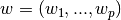 as coef_ and
  as intercept_.
To perform classification with generalized linear models, see Logisitic regression.
3.1.1. Ordinary Least Squares
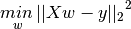
LinearRegression fits a linear model with coefficients
 to minimize the residual sum
of squares between the observed responses in the dataset, and the
responses predicted by the linear approximation. Mathematically it
solves a problem of the form:
to minimize the residual sum
of squares between the observed responses in the dataset, and the
responses predicted by the linear approximation. Mathematically it
solves a problem of the form:

LinearRegression will take in its fit method arrays X, y
and will store the coefficients  of the linear model in its
coef_ member:
of the linear model in its
coef_ member:
>>> from sklearn import linear_model
>>> clf = linear_model.LinearRegression()
>>> clf.fit ([[0, 0], [1, 1], [2, 2]], [0, 1, 2])
LinearRegression(copy_X=True, fit_intercept=True, normalize=False)
>>> clf.coef_
array([ 0.5,  0.5])
However, coefficient estimates for Ordinary Least Squares rely on the
independence of the model terms. When terms are correlated and the
columns of the design matrix  have an approximate linear
dependence, the design matrix becomes close to singular
and as a result, the least-squares estimate becomes highly sensitive
to random errors in the observed response, producing a large
variance. This situation of multicollinearity can arise, for
example, when data are collected without an experimental design.
have an approximate linear
dependence, the design matrix becomes close to singular
and as a result, the least-squares estimate becomes highly sensitive
to random errors in the observed response, producing a large
variance. This situation of multicollinearity can arise, for
example, when data are collected without an experimental design.
Examples:
3.1.1.1. Ordinary Least Squares Complexity
This method computes the least squares solution using a singular value
decomposition of X. If X is a matrix of size (n, p) this method has a
cost of  , assuming that
  .
.
3.1.2. Ridge Regression
Ridge regression addresses some of the problems of Ordinary Least Squares by imposing a penalty on the size of coefficients. The ridge coefficients minimize a penalized residual sum of squares,
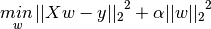
Here,  is a complexity parameter that controls the amount
of shrinkage: the larger the value of
is a complexity parameter that controls the amount
of shrinkage: the larger the value of  , the greater the amount
of shrinkage and thus the coefficients become more robust to collinearity.
, the greater the amount
of shrinkage and thus the coefficients become more robust to collinearity.

As with other linear models, Ridge will take in its fit method
arrays X, y and will store the coefficients of the linear model in
its coef_ member:
>>> from sklearn import linear_model
>>> clf = linear_model.Ridge (alpha = .5)
>>> clf.fit ([[0, 0], [0, 0], [1, 1]], [0, .1, 1])
Ridge(alpha=0.5, copy_X=True, fit_intercept=True, normalize=False, tol=0.001)
>>> clf.coef_
array([ 0.34545455,  0.34545455])
>>> clf.intercept_
0.13636...
Examples:
3.1.2.1. Ridge Complexity
This method has the same order of complexity than an Ordinary Least Squares.
3.1.2.2. Setting the regularization parameter: generalized Cross-Validation
RidgeCV implements ridge regression with built-in cross-validation of the alpha parameter. The object works in the same way as GridSearchCV except that it defaults to Generalized Cross-Validation (GCV), an efficient form of leave-one-out cross-validation:
>>> from sklearn import linear_model
>>> clf = linear_model.RidgeCV(alphas=[0.1, 1.0, 10.0])
>>> clf.fit([[0, 0], [0, 0], [1, 1]], [0, .1, 1])
RidgeCV(alphas=[0.1, 1.0, 10.0], cv=None, fit_intercept=True, loss_func=None,
    normalize=False, score_func=None)
>>> clf.best_alpha
0.1
References
- “Notes on Regularized Least Squares”, Rifkin & Lippert (technical report, course slides).
3.1.3. Lasso
The Lasso is a linear model that estimates sparse coefficients. It is useful in some contexts due to its tendency to prefer solutions with fewer parameter values, effectively reducing the number of variables upon which the given solution is dependent. For this reason, the Lasso and its variants are fundamental to the field of compressed sensing. Under certain conditions, it can recover the exact set of non-zero weights (see Compressive sensing: tomography reconstruction with L1 prior (Lasso)).
Mathematically, it consists of a linear model trained with  prior
as regularizer. The objective function to minimize is:
prior
as regularizer. The objective function to minimize is:
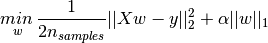
The lasso estimate thus solves the minimization of the
least-squares penalty with  added, where
is a constant and
added, where
is a constant and  is the -norm of
the parameter vector.
is the -norm of
the parameter vector.
The implementation in the class Lasso uses coordinate descent as the algorithm to fit the coefficients. See Least Angle Regression for another implementation:
>>> clf = linear_model.Lasso(alpha = 0.1)
>>> clf.fit([[0, 0], [1, 1]], [0, 1])
Lasso(alpha=0.1, copy_X=True, fit_intercept=True, max_iter=1000,
   normalize=False, precompute='auto', tol=0.0001, warm_start=False)
>>> clf.predict([[1, 1]])
array([ 0.8])
Also useful for lower-level tasks is the function lasso_path that computes the coefficients along the full path of possible values.
Examples:
Note
Feature selection with Lasso
As the Lasso regression yields sparse models, it can thus be used to perform feature selection, as detailed in L1-based feature selection.
3.1.3.1. Setting regularization parameter
The alpha parameter control the degree of sparsity of the coefficients estimated.
3.1.3.1.1. Using cross-validation
scikit-learn exposes objects that set the Lasso alpha parameter by cross-validation: LassoCV and LassoLarsCV. LassoLarsCV is based on the Least Angle Regression algorithm explained below.
For high-dimensional datasets with many collinear regressors, LassoCV is most often preferrable. How, LassoLarsCV has the advantage of exploring more relevant values of alpha parameter, and if the number of samples is very small compared to the number of observations, it is often faster than LassoCV.


3.1.3.1.2. Information-criteria based model selection
Alternatively, the estimator LassoLarsIC proposes to use the Akaike information criterion (AIC) and the Bayes Information criterion (BIC). It is a computationally cheaper alternative to find the optimal value of alpha as the regularization path is computed only once instead of k+1 times when using k-fold cross-validation. However, such criteria needs a proper estimation of the degrees of freedom of the solution, are derived for large samples (asymptotic results) and assume the model is correct, i.e. that the data are actually generated by this model. They also tend to break when the problem is badly conditioned (more features than samples).

3.1.4. Elastic Net
ElasticNet is a linear model trained with L1 and L2 prior as regularizer.
The objective function to minimize is in this case
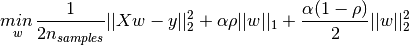

The class ElasticNetCV can be used to set the parameters alpha and rho by cross-validation.
3.1.5. Least Angle Regression
Least-angle regression (LARS) is a regression algorithm for high-dimensional data, developed by Bradley Efron, Trevor Hastie, Iain Johnstone and Robert Tibshirani.
The advantages of LARS are:
- It is numerically efficient in contexts where p >> n (i.e., when the number of dimensions is significantly greater than the number of points)
- It is computationally just as fast as forward selection and has the same order of complexity as an ordinary least squares.
- It produces a full piecewise linear solution path, which is useful in cross-validation or similar attempts to tune the model.
- If two variables are almost equally correlated with the response, then their coefficients should increase at approximately the same rate. The algorithm thus behaves as intuition would expect, and also is more stable.
- It is easily modified to produce solutions for other estimators, like the Lasso.
The disadvantages of the LARS method include:
- Because LARS is based upon an iterative refitting of the residuals, it would appear to be especially sensitive to the effects of noise. This problem is discussed in detail by Weisberg in the discussion section of the Efron et al. (2004) Annals of Statistics article.
The LARS model can be used using estimator Lars, or its low-level implementation lars_path.
3.1.6. LARS Lasso
LassoLars is a lasso model implemented using the LARS algorithm, and unlike the implementation based on coordinate_descent, this yields the exact solution, which is piecewise linear as a function of the norm of its coefficients.

>>> from sklearn import linear_model
>>> clf = linear_model.LassoLars(alpha=.1)
>>> clf.fit([[0, 0], [1, 1]], [0, 1])
LassoLars(alpha=0.1, copy_X=True, eps=..., fit_intercept=True,
     max_iter=500, normalize=True, precompute='auto', verbose=False)
>>> clf.coef_
array([ 0.717157...,  0.        ])
Examples:
The Lars algorithm provides the full path of the coefficients along the regularization parameter almost for free, thus a common operation consist of retrieving the path with function lars_path
3.1.6.1. Mathematical formulation
The algorithm is similar to forward stepwise regression, but instead of including variables at each step, the estimated parameters are increased in a direction equiangular to each one’s correlations with the residual.
Instead of giving a vector result, the LARS solution consists of a curve denoting the solution for each value of the L1 norm of the parameter vector. The full coeffients path is stored in the array coef_path_, which has size (n_features, max_features+1). The first column is always zero.
References:
- Original Algorithm is detailed in the paper Least Angle Regression by Hastie et al.
3.1.7. Orthogonal Matching Pursuit (OMP)
OrthogonalMatchingPursuit and orthogonal_mp implements the OMP algorithm for approximating the fit of a linear model with constraints imposed on the number of non-zero coefficients (ie. the L 0 pseudo-norm).
Being a forward feature selection method like Least Angle Regression, orthogonal matching pursuit can approximate the optimum solution vector with a fixed number of non-zero elements:

Alternatively, orthogonal matching pursuit can target a specific error instead of a specific number of non-zero coefficients. This can be expressed as:

OMP is based on a greedy algorithm that includes at each step the atom most highly correlated with the current residual. It is similar to the simpler matching pursuit (MP) method, but better in that at each iteration, the residual is recomputed using an orthogonal projection on the space of the previously chosen dictionary elements.
Examples:
References:
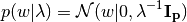
3.1.8. Bayesian Regression
Bayesian regression techniques can be used to include regularization parameters in the estimation procedure: the regularization parameter is not set in a hard sense but tuned to the data at hand.
This can be done by introducing uninformative priors
over the hyper parameters of the model.
The  regularization used in Ridge Regression is equivalent
to finding a maximum a-postiori solution under a Gaussian prior over the
parameters with precision
regularization used in Ridge Regression is equivalent
to finding a maximum a-postiori solution under a Gaussian prior over the
parameters with precision  . Instead of setting
lambda manually, it is possible to treat it as a random variable to be
estimated from the data.
. Instead of setting
lambda manually, it is possible to treat it as a random variable to be
estimated from the data.
To obtain a fully probabilistic model, the output  is assumed
to be Gaussian distributed around
is assumed
to be Gaussian distributed around  :
:

Alpha is again treated as a random variable that is to be estimated from the data.
The advantages of Bayesian Regression are:
- It adapts to the data at hand.
- It can be used to include regularization parameters in the estimation procedure.
The disadvantages of Bayesian regression include:
- Inference of the model can be time consuming.
References
- A good introduction to Bayesian methods is given in C. Bishop: Pattern Recognition and Machine learning
- Original Algorithm is detailed in the book Bayesian learning for neural networks by Radford M. Neal
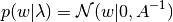
3.1.8.1. Bayesian Ridge Regression
BayesianRidge estimates a probabilistic model of the
regression problem as described above.
The prior for the parameter is given by a spherical Gaussian:
The priors over and  are choosen to be gamma
distributions, the
conjugate prior for the precision of the Gaussian.
are choosen to be gamma
distributions, the
conjugate prior for the precision of the Gaussian.
The resulting model is called Bayesian Ridge Regression, and is similar to the
classical Ridge. The parameters , and
are estimated jointly during the fit of the model. The
remaining hyperparameters are the parameters of the gamma priors over
and . These are usually choosen to be
non-informative. The parameters are estimated by maximizing the marginal
log likelihood.
By default  .
.

Bayesian Ridge Regression is used for regression:
>>> from sklearn import linear_model
>>> X = [[0., 0.], [1., 1.], [2., 2.], [3., 3.]]
>>> Y = [0., 1., 2., 3.]
>>> clf = linear_model.BayesianRidge()
>>> clf.fit(X, Y)
BayesianRidge(alpha_1=1e-06, alpha_2=1e-06, compute_score=False, copy_X=True,
       fit_intercept=True, lambda_1=1e-06, lambda_2=1e-06, n_iter=300,
       normalize=False, tol=0.001, verbose=False)
After being fitted, the model can then be used to predict new values:
>>> clf.predict ([[1, 0.]])
array([ 0.50000013])
The weights of the model can be access:
>>> clf.coef_
array([ 0.49999993,  0.49999993])
Due to the Bayesian framework, the weights found are slightly different to the ones found by Ordinary Least Squares. However, Bayesian Ridge Regression is more robust to ill-posed problem.
Examples:
References
- More details can be found in the article Bayesian Interpolation by MacKay, David J. C.
3.1.8.2. Automatic Relevance Determination - ARD
ARDRegression is very similar to Bayesian Ridge Regression,
but can lead to sparser weights [1].
ARDRegression poses a different prior over , by dropping the
assuption of the Gaussian being spherical.
Instead, the distribution over is assumed to be an axis-parallel,
elliptical Gaussian distribution.
This means each weight  is drawn from a Gaussian distribution,
centered on zero and with a precision
is drawn from a Gaussian distribution,
centered on zero and with a precision  :
:
with  .
.
In constrast to Bayesian Ridge Regression, each coordinate of
has its own standard deviation  . The prior over all
is choosen to be the same gamma distribution given by
hyperparameters
. The prior over all
is choosen to be the same gamma distribution given by
hyperparameters  and
and  .
.

References:
| [1] | David Wipf and Srikantan Nagarajan: A new view of automatic relevance determination. |
3.1.9. Logisitic regression
If the task at hand is to choose which class a sample belongs to given a finite (hopefuly small) set of choices, the learning problem is a classification, rather than regression. Linear models can be used for such a decision, but it is best to use what is called a logistic regression, that doesn’t try to minimize the sum of square residuals, as in regression, but rather a “hit or miss” cost.
The LogisticRegression class can be used to do L1 or L2 penalized logistic regression. L1 penalization yields sparse predicting weights. For L1 penalization sklearn.svm.l1_min_c allows to calculate the lower bound for C in order to get a non “null” (all feature weights to zero) model.
Examples:
- example_linear_model_logistic_l1_l2_sparsity.py
- Path with L1- Logistic Regression
Note
Feature selection with sparse logistic regression
A logistic regression with L1 penalty yields sparse models, and can thus be used to perform feature selection, as detailed in L1-based feature selection.
3.1.10. Stochastic Gradient Descent - SGD
Stochastic gradient descent is a simple yet very efficient approach to fit linear models. It is particulary useful when the number of samples (and the number of features) is very large.
The classes SGDClassifier and SGDRegressor provide functionality to fit linear models for classification and regression using different (convex) loss functions and different penalties.
References
3.1.11. Perceptron
The Perceptron is another simple algorithm suitable for large scale learning. By default:
- It does not require a learning rate.
- It is not regularized (penalized).
- It updates its model only on mistakes.
The last characteristic implies that the Perceptron is slightly faster to train than SGD with the hinge loss and that the resulting models are sparser.