4.2. Clustering
Clustering of unlabeled data can be performed with the module scikits.learn.cluster.
Each clustering algorithm comes in two variants: a class, that implements the fit method to learn the clusters on train data, and a function, that, given train data, returns an array of integer labels corresponding to the different clusters. For the class, the labels over the training data can be found in the labels_ attribute.
Here, we only explain the different algorithms. For usage examples, click on the class name to read the reference documentation.
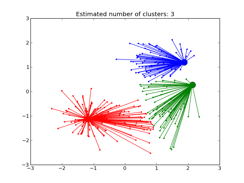
4.2.1. Affinity propagation
AffinityPropagation clusters data by diffusion in the similarity matrix. This algorithm automatically sets its numbers of cluster. It will have difficulties scaling to thousands of samples.
Examples:
- Demo of affinity propagation clustering algorithm: Affinity Propagation on a synthetic 2D datasets with 3 classes.
- Finding structure in the stock market Affinity Propagation on Financial time series to find groups of companies
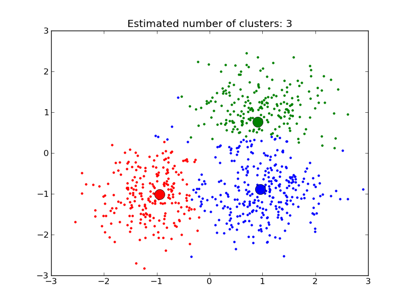
4.2.2. Mean Shift
MeanShift clusters data by estimating blobs in a smooth density of points matrix. This algorithm automatically sets its numbers of cluster. It will have difficulties scaling to thousands of samples.
Examples:
- A demo of the mean-shift clustering algorithm: Mean Shift clustering on a synthetic 2D datasets with 3 classes.
4.2.3. K-means
The KMeans algorithm clusters data by trying to separate samples in n groups of equal variance, minimizing a criterion known as the ‘inertia’ of the groups. This algorithm requires the number of cluster to be specified. It scales well to large number of samples, however its results may be dependent on an initialisation.
4.2.4. Spectral clustering
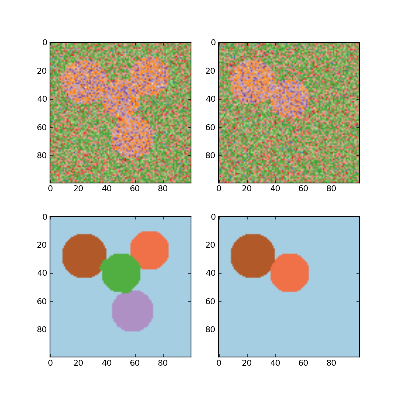
SpectralClustering does an low-dimension embedding of the affinity matrix between samples, followed by a KMeans in the low dimensional space. It is especially efficient if the affinity matrix is sparse and the pyamg module is installed. SpectralClustering requires the number of clusters to be specified. It works well for a small number of clusters but is not advised when using many clusters.
For two clusters, it solves a convex relaxation of the normalised cuts problem on the similarity graph: cutting the graph in two so that the weight of the edges cut is small compared to the weights in of edges inside each cluster. This criteria is especially interesting when working on images: graph vertices are pixels, and edges of the similarity graph are a function of the gradient of the image.
Examples:
- Segmenting the picture of Lena in regions: Spectral clustering to split the image of lena in regions.
- Spectral clustering for image segmentation: Segmenting objects from a noisy background using spectral clustering.