3.2. Support Vector Machines
Support vector machines (SVMs) are a set of supervised learning methods used for classification, regression and outliers detection.
The advantages of Support Vector Machines are:
- Effective in high dimensional spaces.
- Still effective in cases where number of dimensions is greater than the number of samples.
- Uses a subset of training points in the decision function (called support vectors), so it is also memory efficient.
- Versatile: different Kernel functions can be specified for the decision function. Common kernels are provided, but it is also possible to specify custom kernels.
The disadvantages of Support Vector Machines include:
- If the number of features is much greater than the number of samples, the method is likely to give poor performances.
- SVMs do not directly provide probability estimates, these are calculated using five-fold cross-validation, and thus performance can suffer.
3.2.1. Classification
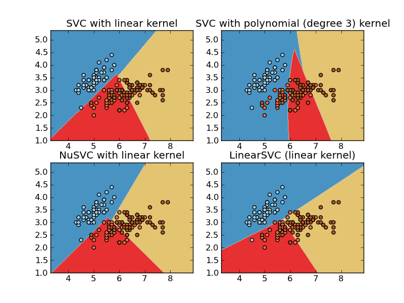
Suppose some given data points each belonging to one of N classes, and the goal is to decide which class a new data point will be in. This problem is called classification, and can be solved with SVMs using Support Vector Classifiers, SVC. The classes that perform this task are SVC, NuSVC and LinearSVC.
SVC and NuSVC are similar methods, but accept slightly different sets of parameters and have different mathematical formulations (see section Mathematical formulation). On the other hand, LinearSVC is another implementation of SVC optimized in the case of a linear kernel. Note that LinearSVC does not accept keyword ‘kernel’, as this is assumed to be linear. It also lacks some of the members of SVC and NuSVC, like support_.
As other classifiers, SVC and NuSVC have to be fitted with two arrays: an array X of size [m_samples, n_features] holding the training samples, and an array Y of size [n_samples] holding the target values (class labels) for the training samples:
>>> from scikits.learn import svm
>>> X = [[0., 0.], [1., 1.]]
>>> Y = [0, 1]
>>> clf = svm.SVC()
>>> clf.fit(X, Y)
SVC(kernel='rbf', C=1.0, probability=False, degree=3, coef0=0.0, eps=0.001,
  cache_size=100.0, shrinking=True, gamma=0.5)
After being fitted, the model can then be used to predict new values:
>>> clf.predict([[2., 2.]])
array([ 1.])
SVMs perform classification as a function of some subset of the training data, called the support vectors. These vectors can be accessed in member support_:
>>> clf.support_
array([0, 1], dtype=int32)
Member n_support_ holds the number of support vectors for each class:
>>> clf.n_support_
array([1, 1], dtype=int32)
3.2.2. Regression
The method of Support Vector Classification can be extended to solve regression problems. This method is called Support Vector Regression.
The model produced by support vector classification (as described above) depends only on a subset of the training data, because the cost function for building the model does not care about training points that lie beyond the margin. Analogously, the model produced by Support Vector Regression depends only on a subset of the training data, because the cost function for building the model ignores any training data close to the model prediction.
There are two flavors of Support Vector Regression: SVR and NuSVR.
As with classification classes, the fit method will take as argument vectors X, y, only that in this case y is expected to have floating point values instead of integer values.
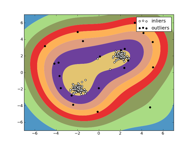
3.2.3. Density estimation, outliers detection
One-class SVM is used for outliers detection, that is, given a set of samples, it will detect the soft boundary of that set so as to classify new points as belonging to that set or not. The class that implements this is called OneClassSVM
In this case, as it is a type of unsupervised learning, the fit method will only take as input an array X, as there are no class labels.
3.2.4. Support Vector machines for sparse data
There is support for sparse data given in any matrix in a format supported by scipy.sparse. Classes have the same name, just prefixed by the sparse namespace, and take the same arguments, with the exception of training and test data, which is expected to be in a matrix format defined in scipy.sparse.
For maximum efficiency, use the CSR matrix format as defined in scipy.sparse.csr_matrix.
Implemented classes are SVC, NuSVC, SVR, NuSVR, OneClassSVM, LinearSVC.
3.2.5. Complexity
Support Vector Machines are powerful tools, but their compute and
storage requirements increase rapidly with the number of training
vectors. The core of an SVM is a quadratic programming problem (QP),
separating support vectors from the rest of the training data. The QP
solver used by this libsvm-based implementation scales between
 and
and
 depending on how efficiently
the libsvm cache is used in practice (dataset dependent). If the data
is very sparse
depending on how efficiently
the libsvm cache is used in practice (dataset dependent). If the data
is very sparse  should be replaced by the average number
of non-zero features in a sample vector.
should be replaced by the average number
of non-zero features in a sample vector.
Also note that for the linear case, the algorithm used in LinearSVC by the liblinear implementation is much more efficient than its libsvm-based SVC counterpart and can scale almost linearly to millions of samples and/or features.
3.2.6. Tips on Practical Use
- Support Vector Machine algorithms are not scale invariant, so it is highly recommended to scale your data. For example, scale each attribute on the input vector X to [0,1] or [-1,+1], or standardize it to have mean 0 and variance 1. Note that the same scaling must be applied to the test vector to obtain meaningful results. See The CookBook for some examples on scaling.
- Parameter nu in NuSVC/OneClassSVM/NuSVR approximates the fraction of training errors and support vectors.
- If data for classification are unbalanced (e.g. many positive and few negative), set class_weight=’auto’ and/or try different penalty parameters C.
- Specify larger cache size (keyword cache) for huge problems.
- The underlying LinearSVC implementation uses a random number generator to select features when fitting the model. It is thus not uncommon, to have slightly different results for the same input data. If that happens, try with a smaller eps parameter.
3.2.7. Kernel functions
The kernel function can be any of the following:
- linear:
.
- polynomial:
. d is specified by keyword degree.
- rbf (
).
is specified by keyword gamma.
- sigmoid (
).
Different kernels are specified by keyword kernel at initialization:
>>> linear_svc = svm.SVC(kernel='linear')
>>> linear_svc.kernel
'linear'
>>> rbf_svc = svm.SVC(kernel='rbf')
>>> rbf_svc.kernel
'rbf'
3.2.7.1. Custom Kernels
You can define your own kernels by either giving the kernel as a python function or by precomputing the Gram matrix.
Classifiers with custom kernels behave the same way as any other classifiers, except that:
- Field support_vectors_ is now empty, only indices of support vectors are stored in support_
- A reference (and not a copy) of the first argument in the fit() method is stored for future reference. If that array changes between the use of fit() and predict() you will have unexpected results.
3.2.7.1.1. Using python functions as kernels
You can also use your own defined kernels by passing a function to the keyword kernel in the constructor.
Your kernel must take as arguments two matrices and return a third matrix.
The following code defines a linear kernel and creates a classifier instance that will use that kernel:
>>> import numpy as np
>>> from scikits.learn import svm
>>> def my_kernel(x, y):
...     return np.dot(x, y.T)
...
>>> clf = svm.SVC(kernel=my_kernel)
3.2.7.1.2. Using the Gram matrix
Set kernel=’precomputed’ and pass the Gram matrix instead of X in the fit method.
Examples:
3.2.8. Mathematical formulation
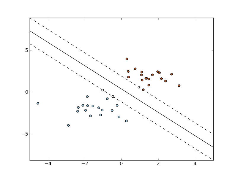
A support vector machine constructs a hyper-plane or set of hyper-planes in a high or infinite dimensional space, which can be used for classification, regression or other tasks. Intuitively, a good separation is achieved by the hyper-plane that has the largest distance to the nearest training data points of any class (so-called functional margin), since in general the larger the margin the lower the generalization error of the classifier.
3.2.8.1. SVC
Given training vectors  , i=1,..., l, in two
classes, and a vector
, i=1,..., l, in two
classes, and a vector  such that
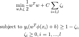
  , SVC solves the following primal problem:
Its dual is
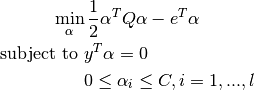
where  is the vector of all ones, C > 0 is the upper bound, Q
is an l by l positive semidefinite matrix,
is the vector of all ones, C > 0 is the upper bound, Q
is an l by l positive semidefinite matrix, 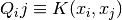 and
and  is the kernel. Here training
vectors are mapped into a higher (maybe infinite) dimensional space by
the function
is the kernel. Here training
vectors are mapped into a higher (maybe infinite) dimensional space by
the function 
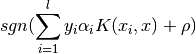
The decision function is:
This parameters can be accessed through the members dual_coef_
which holds the product  , support_vectors_ which
holds the support vectors, and intercept_ which holds the independent
term
, support_vectors_ which
holds the support vectors, and intercept_ which holds the independent
term  :
:
References:
- “Automatic Capacity Tuning of Very Large VC-dimension Classifiers” I Guyon, B Boser, V Vapnik - Advances in neural information processing 1993,
- “Support-vector networks” C. Cortes, V. Vapnik, Machine Leaming, 20, 273-297 (1995)
3.2.8.2. NuSVC
We introduce a new parameter  which controls the number of
support vectors and training errors. The parameter
which controls the number of
support vectors and training errors. The parameter ![\nu \in (0,
1]](../_images/math/948360fd417f20a48ae449aa26ede1baef981854.png) is an upper bound on the fraction of training errors and a lower
bound of the fraction of support vectors.
is an upper bound on the fraction of training errors and a lower
bound of the fraction of support vectors.
3.2.9. Frequently Asked Questions
Q: Can I get the indices of the support vectors instead of the support vectors ?
A: The underlying C implementation does not provide this information.