Ledoit-Wolf vs Covariance simple estimation¶

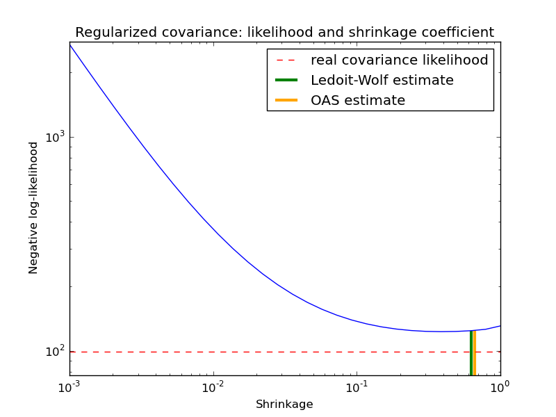
The usual covariance maximum likelihood estimate can be regularized using shrinkage. Ledoit and Wolf proposed a close formula to compute the asymptotical optimal shrinkage parameter (minimizing a MSE criterion), yielding the Ledoit-Wolf covariance estimate.

Chen et al. proposed an improvement of the Ledoit-Wolf shrinkage parameter, the OAS coefficient, whose convergence is significantly better under the assumption that the data are gaussian.

In this example, we compute the likelihood of unseen data for different values of the shrinkage parameter, highlighting the LW and OAS estimates. The Ledoit-Wolf estimate stays close to the likelihood criterion optimal value, which is an artifact of the method since it is asymptotic and we are working with a small number of observations. The OAS estimate deviates from the likelihood criterion optimal value but better approximate the MSE optimal value, especially for a small number a observations.

../../_images/plot_covariance_estimation_1.png

Python source code: plot_covariance_estimation.py

print __doc__

import numpy as np
import pylab as pl
from scipy import linalg

###############################################################################
# Generate sample data
n_features, n_samples = 30, 20
base_X_train = np.random.normal(size=(n_samples, n_features))
base_X_test = np.random.normal(size=(n_samples, n_features))

# Color samples
coloring_matrix = np.random.normal(size=(n_features, n_features))
X_train = np.dot(base_X_train, coloring_matrix)
X_test = np.dot(base_X_test, coloring_matrix)

###############################################################################
# Compute Ledoit-Wolf and Covariances on a grid of shrinkages

from sklearn.covariance import LedoitWolf, OAS, ShrunkCovariance, \
    log_likelihood, empirical_covariance

# Ledoit-Wolf optimal shrinkage coefficient estimate
lw = LedoitWolf()
loglik_lw = lw.fit(X_train, assume_centered=True).score(
    X_test, assume_centered=True)

# OAS coefficient estimate
oa = OAS()
loglik_oa = oa.fit(X_train, assume_centered=True).score(
    X_test, assume_centered=True)

# spanning a range of possible shrinkage coefficient values
shrinkages = np.logspace(-3, 0, 30)
negative_logliks = [-ShrunkCovariance(shrinkage=s).fit(
        X_train, assume_centered=True).score(X_test, assume_centered=True) \
                         for s in shrinkages]

# getting the likelihood under the real model
real_cov = np.dot(coloring_matrix.T, coloring_matrix)
emp_cov = empirical_covariance(X_train)
loglik_real = -log_likelihood(emp_cov, linalg.inv(real_cov))

###############################################################################
# Plot results
pl.figure()
pl.title("Regularized covariance: likelihood and shrinkage coefficient")
pl.xlabel('Shrinkage')
pl.ylabel('Negative log-likelihood')
# range shrinkage curve
pl.loglog(shrinkages, negative_logliks)

# real likelihood reference
# BUG: hlines(..., linestyle='--') breaks on some older versions of matplotlib
#pl.hlines(loglik_real, pl.xlim()[0], pl.xlim()[1], color='red',
#          label="real covariance likelihood", linestyle='--')
pl.plot(pl.xlim(), 2 * [loglik_real], '--r',
        label="real covariance likelihood")

# adjust view
lik_max = np.amax(negative_logliks)
lik_min = np.amin(negative_logliks)
ylim0 = lik_min - 5. * np.log((pl.ylim()[1] - pl.ylim()[0]))
ylim1 = lik_max + 10. * np.log(lik_max - lik_min)
# LW likelihood
pl.vlines(lw.shrinkage_, ylim0, -loglik_lw, color='g',
          linewidth=3, label='Ledoit-Wolf estimate')
# OAS likelihood
pl.vlines(oa.shrinkage_, ylim0, -loglik_oa, color='orange',
          linewidth=3, label='OAS estimate')

pl.ylim(ylim0, ylim1)
pl.xlim(shrinkages[0], shrinkages[-1])
pl.legend()
pl.show()

Citing

This page

Ledoit-Wolf vs Covariance simple estimation¶