Robust vs Empirical covariance estimate
The usual covariance maximum likelihood estimate is very sensitive to the presence of outliers in the data set. In such a case, one would have better to use a robust estimator of covariance to garanty that the estimation is resistant to “errorneous” observations in the data set.
The Minimum Covariance Determinant estimator is a robust, high-breakdown point (i.e. it can be used to estimate the covariance matrix of highly contaminated datasets, up to :math:` rac{n_samples-n_features-1}{2}` outliers) estimator of covariance. The idea is to find :math:` rac{n_samples+n_features+1}{2}` observations whose empirical covariance has the smallest determinant, yielding a “pure” subset of observations from which to compute standards estimates of location and covariance. After a correction step aiming at compensating the fact the the estimates were learnt from only a portion of the initial data, we end up with robust estimates of the data set location and covariance.
The Minimum Covariance Determinant estimator (MCD) has been introduced by P.J.Rousseuw in [1].
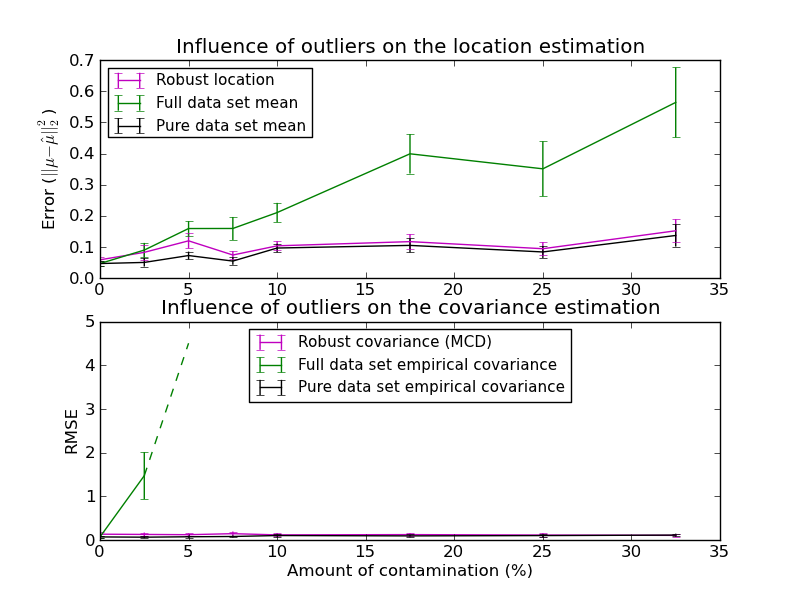
In this example, we compare the estimation errors that are made when using three types of location and covariance estimates on contaminated gaussian distributed data sets:
- The mean and the empirical covariance of the full dataset, which break down as soon as there are outliers in the data set
- The robust MCD, that has a low error provided n_samples > 5 * n_features
- The mean and the empirical covariance of the observations that are known to be good ones. This can be considered as a “perfect” MCD estimation, so one can trust our implementation by comparing to this case.
- [1] P. J. Rousseeuw. Least median of squares regression. J. Am
- Stat Ass, 79:871, 1984.
- [2] Johanna Hardin, David M Rocke. Journal of Computational and
- Graphical Statistics. December 1, 2005, 14(4): 928-946.
Python source code: plot_robust_vs_empirical_covariance.py
print __doc__

import numpy as np
import pylab as pl
import matplotlib.font_manager

from sklearn.covariance import EmpiricalCovariance, MinCovDet

# example settings
n_samples = 80
n_features = 5
repeat = 10

range_n_outliers = np.concatenate(
    (np.linspace(0, n_samples / 8, 5),
     np.linspace(n_samples / 8, n_samples / 2, 5)[1:-1]))

# definition of arrays to store results
err_loc_mcd = np.zeros((range_n_outliers.size, repeat))
err_cov_mcd = np.zeros((range_n_outliers.size, repeat))
err_loc_emp_full = np.zeros((range_n_outliers.size, repeat))
err_cov_emp_full = np.zeros((range_n_outliers.size, repeat))
err_loc_emp_pure = np.zeros((range_n_outliers.size, repeat))
err_cov_emp_pure = np.zeros((range_n_outliers.size, repeat))

# computation
for i, n_outliers in enumerate(range_n_outliers):
    for j in range(repeat):
        # generate data
        X = np.random.randn(n_samples, n_features)
        # add some outliers
        outliers_index = np.random.permutation(n_samples)[:n_outliers]
        outliers_offset = 10. * \
            (np.random.randint(2, size=(n_outliers, n_features)) - 0.5)
        X[outliers_index] += outliers_offset
        inliers_mask = np.ones(n_samples).astype(bool)
        inliers_mask[outliers_index] = False

        # fit a Minimum Covariance Determinant (MCD) robust estimator to data
        S = MinCovDet().fit(X)
        # compare raw robust estimates with the true location and covariance
        err_loc_mcd[i, j] = np.sum(S.location_ ** 2)
        err_cov_mcd[i, j] = S.error_norm(np.eye(n_features))
        # compare estimators learnt from the full data set with true parameters
        err_loc_emp_full[i, j] = np.sum(X.mean(0) ** 2)
        err_cov_emp_full[i, j] = EmpiricalCovariance().fit(X).error_norm(
            np.eye(n_features))
        # compare with an empirical covariance learnt from a pure data set
        # (i.e. "perfect" MCD)
        pure_X = X[inliers_mask]
        pure_location = pure_X.mean(0)
        pure_emp_cov = EmpiricalCovariance().fit(pure_X)
        err_loc_emp_pure[i, j] = np.sum(pure_location ** 2)
        err_cov_emp_pure[i, j] = pure_emp_cov.error_norm(np.eye(n_features))

# Display results
font_prop = matplotlib.font_manager.FontProperties(size=11)
pl.subplot(2, 1, 1)
pl.errorbar(range_n_outliers, err_loc_mcd.mean(1),
            yerr=err_loc_mcd.std(1) / np.sqrt(repeat),
            label="Robust location", color='m')
pl.errorbar(range_n_outliers, err_loc_emp_full.mean(1),
            yerr=err_loc_emp_full.std(1) / np.sqrt(repeat),
            label="Full data set mean", color='green')
pl.errorbar(range_n_outliers, err_loc_emp_pure.mean(1),
            yerr=err_loc_emp_pure.std(1) / np.sqrt(repeat),
            label="Pure data set mean", color='black')
pl.title("Influence of outliers on the location estimation")
pl.ylabel(r"Error ($||\mu - \hat{\mu}||_2^2$)")
pl.legend(loc="upper left", prop=font_prop)

pl.subplot(2, 1, 2)
x_size = range_n_outliers.size
pl.errorbar(range_n_outliers, err_cov_mcd.mean(1),
            yerr=err_cov_mcd.std(1),
            label="Robust covariance (MCD)", color='m')
pl.errorbar(range_n_outliers[:(x_size / 5 + 1)],
            err_cov_emp_full.mean(1)[:(x_size / 5 + 1)],
            yerr=err_cov_emp_full.std(1)[:(x_size / 5 + 1)],
            label="Full data set empirical covariance", color='green')
pl.plot(range_n_outliers[(x_size / 5):(x_size / 2 - 1)],
         err_cov_emp_full.mean(1)[(x_size / 5):(x_size / 2 - 1)],
         color='green', ls='--')
pl.errorbar(range_n_outliers, err_cov_emp_pure.mean(1),
            yerr=err_cov_emp_pure.std(1),
            label="Pure data set empirical covariance", color='black')
pl.title("Influence of outliers on the covariance estimation")
pl.xlabel("Amount of contamination (%)")
pl.ylabel("RMSE")
pl.legend(loc="upper center", prop=font_prop)

pl.show()