Bayesian Ridge Regression
Computes a Bayesian Ridge Regression on a synthetic dataset.
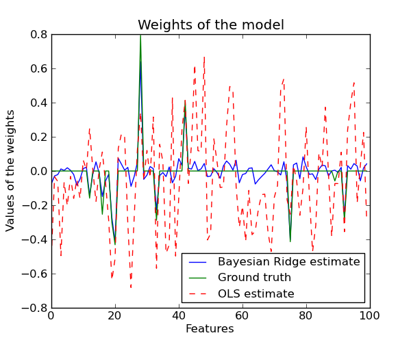
Compared to the OLS (ordinary least squares) estimator, the coefficient weights are slightly shifted toward zeros, wich stabilises them.
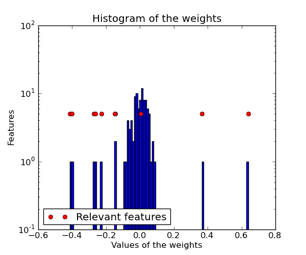
As the prior on the weights is a Gaussian prior, the histogram of the estimated weights is Gaussian.
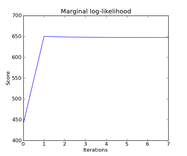
The estimation of the model is done by iteratively maximizing the marginal log-likelihood of the observations.
Python source code: plot_bayesian_ridge.py
print __doc__

import numpy as np
import pylab as pl
from scipy import stats

from sklearn.linear_model import BayesianRidge, LinearRegression

###############################################################################
# Generating simulated data with Gaussian weigthts
np.random.seed(0)
n_samples, n_features = 100, 100
X = np.random.randn(n_samples, n_features)  # Create gaussian data
# Create weigts with a precision lambda_ of 4.
lambda_ = 4.
w = np.zeros(n_features)
# Only keep 10 weights of interest
relevant_features = np.random.randint(0, n_features, 10)
for i in relevant_features:
    w[i] = stats.norm.rvs(loc=0, scale=1. / np.sqrt(lambda_))
# Create noise with a precision alpha of 50.
alpha_ = 50.
noise = stats.norm.rvs(loc=0, scale=1. / np.sqrt(alpha_), size=n_samples)
# Create the target
y = np.dot(X, w) + noise

###############################################################################
# Fit the Bayesian Ridge Regression and an OLS for comparison
clf = BayesianRidge(compute_score=True)
clf.fit(X, y)

ols = LinearRegression()
ols.fit(X, y)

###############################################################################
# Plot true weights, estimated weights and histogram of the weights
pl.figure(figsize=(6, 5))
pl.title("Weights of the model")
pl.plot(clf.coef_, 'b-', label="Bayesian Ridge estimate")
pl.plot(w, 'g-', label="Ground truth")
pl.plot(ols.coef_, 'r--', label="OLS estimate")
pl.xlabel("Features")
pl.ylabel("Values of the weights")
pl.legend(loc="best", prop=dict(size=12))

pl.figure(figsize=(6, 5))
pl.title("Histogram of the weights")
pl.hist(clf.coef_, bins=n_features, log=True)
pl.plot(clf.coef_[relevant_features], 5 * np.ones(len(relevant_features)),
        'ro', label="Relevant features")
pl.ylabel("Features")
pl.xlabel("Values of the weights")
pl.legend(loc="lower left")

pl.figure(figsize=(6, 5))
pl.title("Marginal log-likelihood")
pl.plot(clf.scores_)
pl.ylabel("Score")
pl.xlabel("Iterations")
pl.show()