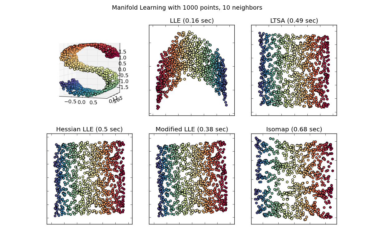
Comparison of Manifold Learning methods

An illustration of dimensionality reduction on the S-curve dataset with various manifold learning methods.

For a discussion and comparison of these algorithms, see the manifold module page

Script output:

standard: 0.16 sec
ltsa: 0.49 sec
hessian: 0.5 sec
modified: 0.38 sec
Isomap: 0.68 sec

Python source code: plot_compare_methods.py

# Author: Jake Vanderplas -- <vanderplas@astro.washington.edu>

print __doc__

from time import time

import pylab as pl
from mpl_toolkits.mplot3d import Axes3D
from matplotlib.ticker import NullFormatter

from sklearn import manifold, datasets

n_points = 1000
X, color = datasets.samples_generator.make_s_curve(n_points)
n_neighbors = 10
out_dim = 2

fig = pl.figure(figsize=(12, 8))
pl.suptitle("Manifold Learning with %i points, %i neighbors"
               % (1000, n_neighbors), fontsize=14)

try:
    # compatibility matplotlib < 1.0
    ax = fig.add_subplot(231, projection='3d')
    ax.scatter(X[:, 0], X[:, 1], X[:, 2], c=color, cmap=pl.cm.Spectral)
    ax.view_init(4, -72)
except:
    ax = fig.add_subplot(231, projection='3d')
    pl.scatter(X[:, 0], X[:, 2], c=color, cmap=pl.cm.Spectral)

methods = ['standard', 'ltsa', 'hessian', 'modified']
labels = ['LLE', 'LTSA', 'Hessian LLE', 'Modified LLE']

for i, method in enumerate(methods):
    t0 = time()
    Y = manifold.LocallyLinearEmbedding(n_neighbors, out_dim,
                                        eigen_solver='auto',
                                        method=method).fit_transform(X)
    t1 = time()
    print "%s: %.2g sec" % (methods[i], t1 - t0)

    ax = fig.add_subplot(232 + i)
    pl.scatter(Y[:, 0], Y[:, 1], c=color, cmap=pl.cm.Spectral)
    pl.title("%s (%.2g sec)" % (labels[i], t1 - t0))
    ax.xaxis.set_major_formatter(NullFormatter())
    ax.yaxis.set_major_formatter(NullFormatter())
    pl.axis('tight')

t0 = time()
Y = manifold.Isomap(n_neighbors, out_dim).fit_transform(X)
t1 = time()
print "Isomap: %.2g sec" % (t1 - t0)
ax = fig.add_subplot(236)
pl.scatter(Y[:, 0], Y[:, 1], c=color, cmap=pl.cm.Spectral)
pl.title("Isomap (%.2g sec)" % (t1 - t0))
ax.xaxis.set_major_formatter(NullFormatter())
ax.yaxis.set_major_formatter(NullFormatter())
pl.axis('tight')

pl.show()