4.2. Manifold learning¶

Look for the bare necessities
The simple bare necessities
Forget about your worries and your strife
I mean the bare necessities
Old Mother Nature’s recipes
That bring the bare necessities of life

– Baloo’s song [The Jungle Book]

Manifold learning is an approach to nonlinear dimensionality reduction. Algorithms for this task are based on the idea that the dimensionality of many data sets is only artificially high.

4.2.1. Introduction¶

High-dimensional datasets can be very difficult to visualize. While data in two or three dimensions can be plotted to show the inherent structure of the data, equivalent high-dimensional plots are much less intuitive. To aid visualization of the structure of a dataset, the dimension must be reduced in some way.

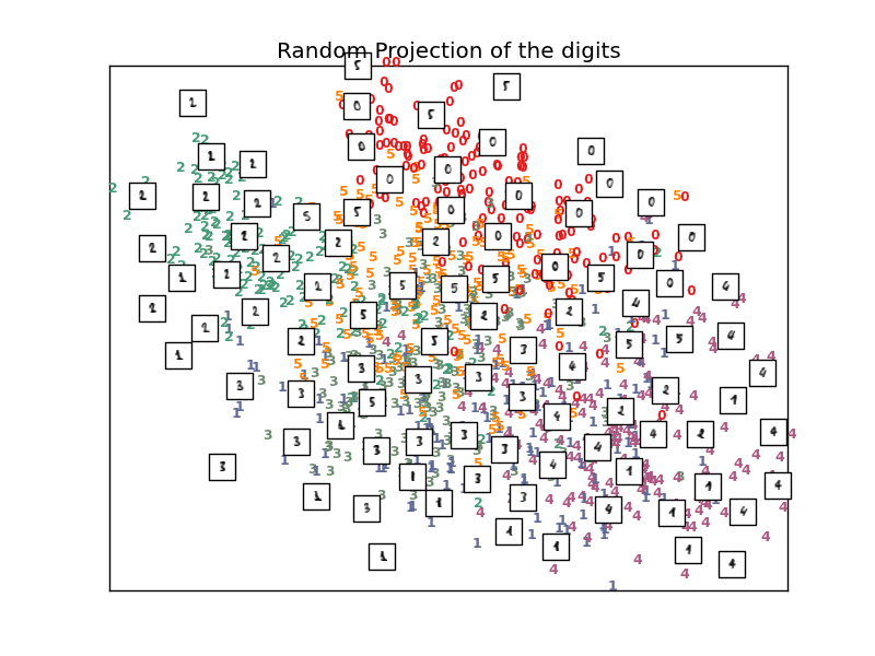
The simplest way to accomplish this dimensionality reduction is by taking a random projection of the data. Though this allows some degree of visualization of the data structure, the randomness of the choice leaves much to be desired. In a random projection, it is likely that the more interesting structure within the data will be lost.

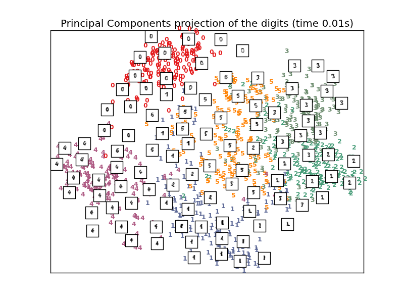
To address this concern, a number of supervised and unsupervised linear dimensionality reduction frameworks have been designed, such as Principal Component Analysis (PCA), Independent Component Analysis, Linear Discriminant Analysis, and others. These algorithms define specific rubrics to choose an “interesting” linear projection of the data. These methods can be powerful, but often miss important nonlinear structure in the data.

Manifold Learning can be thought of as an attempt to generalize linear frameworks like PCA to be sensitive to nonlinear structure in data. Though supervised variants exist, the typical manifold learning problem is unsupervised: it learns the high-dimensional structure of the data from the data itself, without the use of predetermined classifications.

Examples:

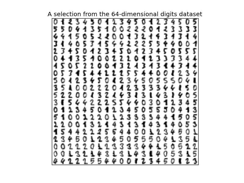
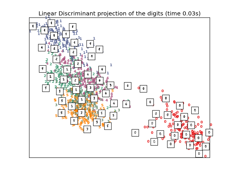
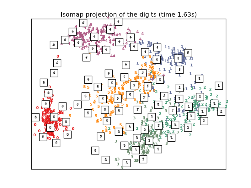
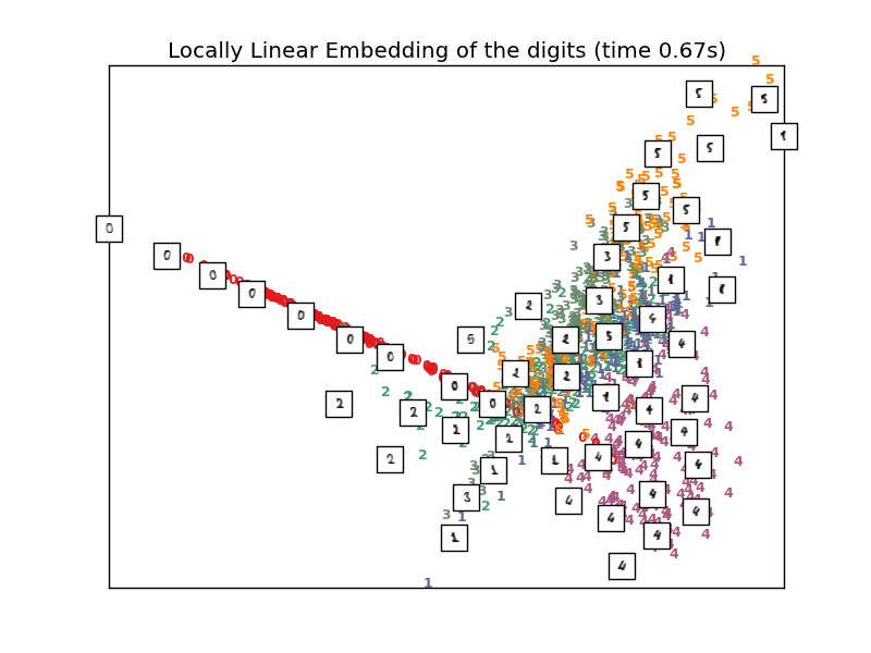
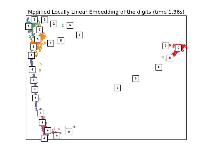
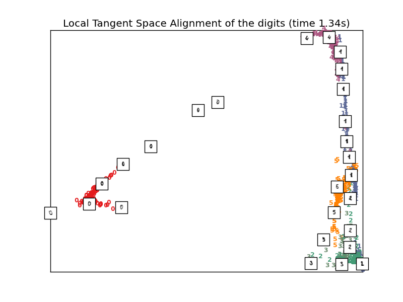
See Manifold learning on handwritten digits: Locally Linear Embedding, Isomap... for an example of dimensionality reduction on handwritten digits.
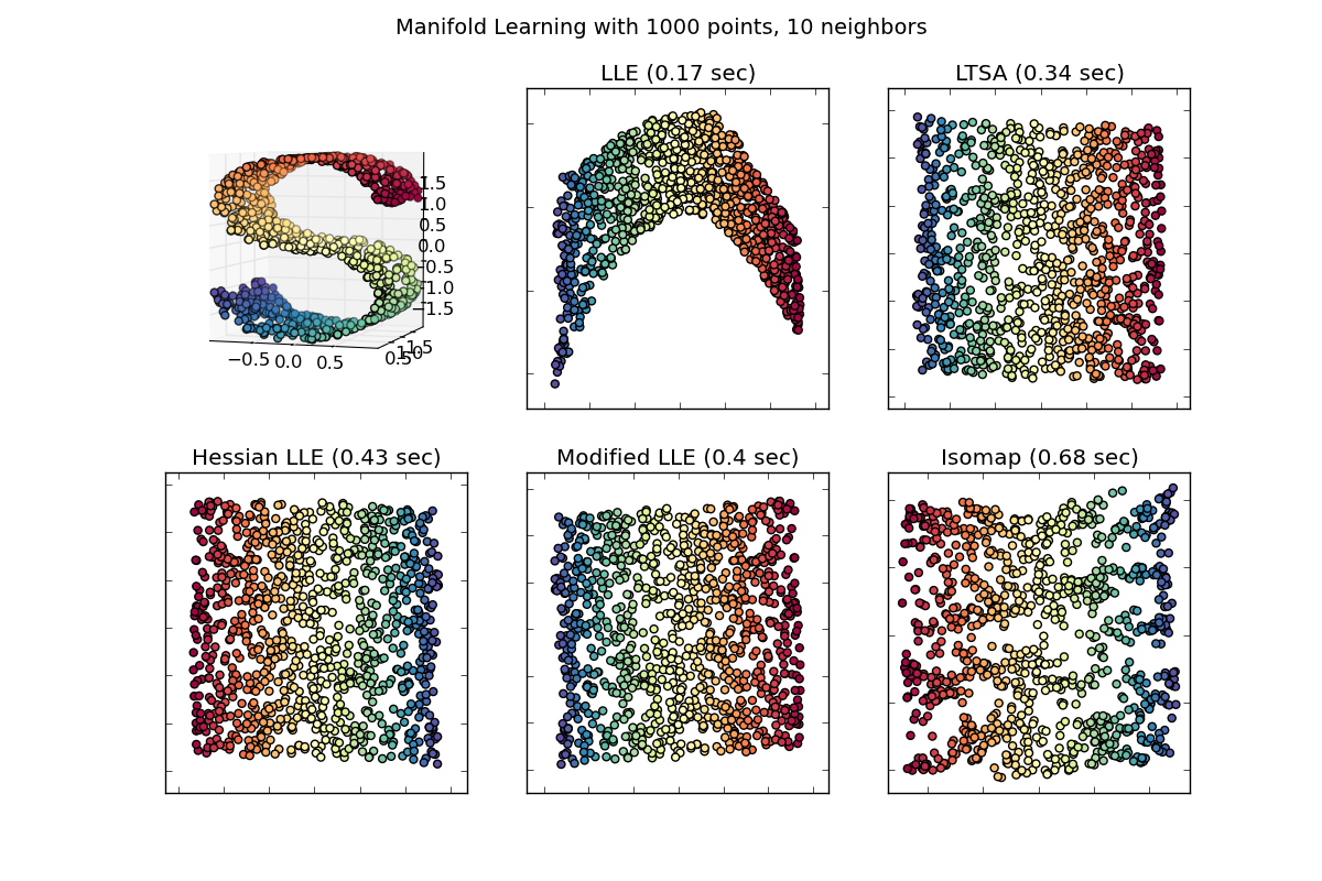
See Comparison of Manifold Learning methods for an example of dimensionality reduction on a toy “S-curve” dataset.

The manifold learning implementations available in sklearn are summarized below

4.2.2. Isomap¶

One of the earliest approaches to manifold learning is the Isomap algorithm, short for Isometric Mapping. Isomap can be viewed as an extension of Multi-dimensional Scaling (MDS) or Kernel PCA. Isomap seeks a lower-dimensional embedding which maintains geodesic distances between all points. Isomap can be performed with the object Isomap.

4.2.2.1. Complexity¶

The Isomap algorithm comprises three stages:

Nearest neighbor search. Isomap uses sklearn.neighbors.BallTree for efficient neighbor search. The cost is approximately $O[D \log(k) N \log(N)]$ , for $k$ nearest neighbors of $N$ points in $D$ dimensions.
Shortest-path graph search. The most efficient known algorithms for this are Dijkstra’s Algorithm, which is approximately $O[N^2(k + \log(N))]$ , or the Floyd-Warshall algorithm, which is $O[N^3]$ . The algorithm can be selected by the user with the path_method keyword of Isomap. If unspecified, the code attempts to choose the best algorithm for the input data.
Partial eigenvalue decomposition. The embedding is encoded in the eigenvectors corresponding to the $d$ largest eigenvalues of the $N \times N$ isomap kernel. For a dense solver, the cost is approximately $O[d N^2]$ . This cost can often be improved using the ARPACK solver. The eigensolver can be specified by the user with the path_method keyword of Isomap. If unspecified, the code attempts to choose the best algorithm for the input data.

The overall complexity of Isomap is $O[D \log(k) N \log(N)] + O[N^2(k + \log(N))] + O[d N^2]$ .

$N$ : number of training data points
$D$ : input dimension
$k$ : number of nearest neighbors
$d$ : output dimension

References:

“A global geometric framework for nonlinear dimensionality reduction” Tenenbaum, J.B.; De Silva, V.; & Langford, J.C. Science 290 (5500)

4.2.3. Locally Linear Embedding¶

Locally linear embedding (LLE) seeks a lower-dimensional projection of the data which preserves distances within local neighborhoods. It can be thought of as a series of local Principal Component Analyses which are globally compared to find the best nonlinear embedding.

Locally linear embedding can be performed with function locally_linear_embedding or its object-oriented counterpart LocallyLinearEmbedding.

4.2.3.1. Complexity¶

The standard LLE algorithm comprises three stages:

Nearest Neighbors Search. See discussion under Isomap above.
Weight Matrix Construction. $O[D N k^3]$ . The construction of the LLE weight matrix involves the solution of a $k \times k$ linear equation for each of the $N$ local neighborhoods
Partial Eigenvalue Decomposition. See discussion under Isomap above.

The overall complexity of standard LLE is $O[D \log(k) N \log(N)] + O[D N k^3] + O[d N^2]$ .

$N$ : number of training data points
$D$ : input dimension
$k$ : number of nearest neighbors
$d$ : output dimension

References:

“Nonlinear dimensionality reduction by locally linear embedding” Roweis, S. & Saul, L. Science 290:2323 (2000)

4.2.4. Modified Locally Linear Embedding¶

One well-known issue with LLE is the regularization problem. When the number of neighbors is greater than the number of input dimensions, the matrix defining each local neighborhood is rank-deficient. To address this, standard LLE applies an arbitrary regularization parameter $r$ , which is chosen relative to the trace of the local weight matrix. Though it can be shown formally that as $r \to 0$ , the solution coverges to the desired embedding, there is no guarantee that the optimal solution will be found for $r > 0$ . This problem manifests itself in embeddings which distort the underlying geometry of the manifold.

One method to address the regularization problem is to use multiple weight vectors in each neighborhood. This is the essence of modified locally linear embedding (MLLE). MLLE can be performed with function locally_linear_embedding or its object-oriented counterpart LocallyLinearEmbedding, with the keyword method = 'modified'. It requires n_neighbors > out_dim.

4.2.4.1. Complexity¶

The MLLE algorithm comprises three stages:

Nearest Neighbors Search. Same as standard LLE
Weight Matrix Construction. Approximately $O[D N k^3] + O[N (k-D) k^2]$ . The first term is exactly equivalent to that of standard LLE. The second term has to do with constructing the weight matrix from multiple weights. In practice, the added cost of constructing the MLLE weight matrix is relatively small compared to the cost of steps 1 and 3.
Partial Eigenvalue Decomposition. Same as standard LLE

The overall complexity of MLLE is $O[D \log(k) N \log(N)] + O[D N k^3] + O[N (k-D) k^2] + O[d N^2]$ .

$N$ : number of training data points
$D$ : input dimension
$k$ : number of nearest neighbors
$d$ : output dimension

References:

“MLLE: Modified Locally Linear Embedding Using Multiple Weights” Zhang, Z. & Wang, J.

4.2.5. Hessian Eigenmapping¶

Hessian Eigenmapping (also known as Hessian-based LLE: HLLE) is another method of solving the regularization problem of LLE. It revolves around a hessian-based quadratic form at each neighborhood which is used to recover the locally linear structure. Though other implementations note its poor scaling with data size, sklearn implements some algorithmic improvements which make its cost comparable to that of other LLE variants for small output dimension. HLLE can be performed with function locally_linear_embedding or its object-oriented counterpart LocallyLinearEmbedding, with the keyword method = 'hessian'. It requires n_neighbors > out_dim * (out_dim + 3) / 2.

4.2.5.1. Complexity¶

The HLLE algorithm comprises three stages:

Nearest Neighbors Search. Same as standard LLE
Weight Matrix Construction. Approximately $O[D N k^3] + O[N d^6]$ . The first term reflects a similar cost to that of standard LLE. The second term comes from a QR decomposition of the local hessian estimator.
Partial Eigenvalue Decomposition. Same as standard LLE

The overall complexity of standard HLLE is $O[D \log(k) N \log(N)] + O[D N k^3] + O[N d^6] + O[d N^2]$ .

$N$ : number of training data points
$D$ : input dimension
$k$ : number of nearest neighbors
$d$ : output dimension

References:

“Hessian Eigenmaps: Locally linear embedding techniques for high-dimensional data” Donoho, D. & Grimes, C. Proc Natl Acad Sci USA. 100:5591 (2003)

4.2.6. Local Tangent Space Alignment¶

Though not technically a variant of LLE, Local tangent space alignment (LTSA) is algorithmically similar enough to LLE that it can be put in this category. Rather than focusing on preserving neighborhood distances as in LLE, LTSA seeks to characterize the local geometry at each neighborhood via its tangent space, and performs a global optimization to align these local tangent spaces to learn the embedding. LTSA can be performed with function locally_linear_embedding or its object-oriented counterpart LocallyLinearEmbedding, with the keyword method = 'ltsa'.

4.2.6.1. Complexity¶

The LTSA algorithm comprises three stages:

Nearest Neighbors Search. Same as standard LLE
Weight Matrix Construction. Approximately $O[D N k^3] + O[k^2 d]$ . The first term reflects a similar cost to that of standard LLE.
Partial Eigenvalue Decomposition. Same as standard LLE

The overall complexity of standard LTSA is $O[D \log(k) N \log(N)] + O[D N k^3] + O[k^2 d] + O[d N^2]$ .

$N$ : number of training data points
$D$ : input dimension
$k$ : number of nearest neighbors
$d$ : output dimension

References:

“Principal manifolds and nonlinear dimensionality reduction via tangent space alignment” Zhang, Z. & Zha, H. Journal of Shanghai Univ. 8:406 (2004)

4.2.7. Tips on practical use¶

Make sure the same scale is used over all features. Because manifold learning methods are based on a nearest-neighbor search, the algorithm may perform poorly otherwise. See Scaler for convenient ways of scaling heterogeneous data.
The reconstruction error computed by each routine can be used to choose the optimal output dimension. For a $d$ -dimensional manifold embedded in a $D$ -dimensional parameter space, the reconstruction error will decrease as out_dim is increased until out_dim == d.
Note that noisy data can “short-circuit” the manifold, in essence acting as a bridge between parts of the manifold that would otherwise be well-separated. Manifold learning on noisy and/or incomplete data is an active area of research.
Certain input configurations can lead to singular weight matrices, for example when more than two points in the dataset are identical, or when the data is split into disjointed groups. In this case, method='arpack' will fail to find the null space. The easiest way to address this is to use method='dense' which will work on a singular matrix, though it may be very slow depending on the number of input points. Alternatively, one can attempt to understand the source of the singularity: if it is due to disjoint sets, increasing n_neighbors may help. If it is due to identical points in the dataset, removing these points may help.

Citing

This page

4.2. Manifold learning¶

4.2.1. Introduction¶

4.2.2. Isomap¶

4.2.2.1. Complexity¶

4.2.3. Locally Linear Embedding¶

4.2.3.1. Complexity¶

4.2.4. Modified Locally Linear Embedding¶

4.2.4.1. Complexity¶

4.2.5. Hessian Eigenmapping¶

4.2.5.1. Complexity¶

4.2.6. Local Tangent Space Alignment¶

4.2.6.1. Complexity¶

4.2.7. Tips on practical use¶