SVM-Kernels
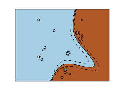
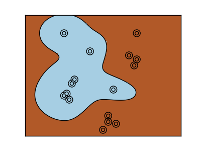
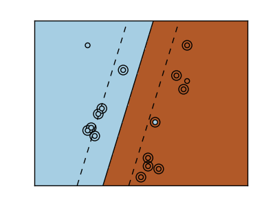
Three different types of SVM-Kernels are displayed below. The polynomial and RBF are especially useful when the data-points are not linearly seperable.
Python source code: plot_svm_kernels.py
print __doc__


# Code source: Gael Varoqueux
# License: BSD

import numpy as np
import pylab as pl
from sklearn import svm


# Our dataset and targets
X = np.c_[(.4, -.7),
          (-1.5, -1),
          (-1.4, -.9),
          (-1.3, -1.2),
          (-1.1, -.2),
          (-1.2, -.4),
          ( -.5,  1.2),
          ( -1.5,  2.1),
          ( 1,  1),
          # --
          ( 1.3,  .8),
          ( 1.2,  .5),
          ( .2,  -2),
          ( .5,  -2.4),
          ( .2,  -2.3),
          ( 0,  -2.7),
          ( 1.3,  2.1),
         ].T
Y = [0]*8 + [1]*8

# figure number
fignum = 1

# fit the model
for kernel in ('linear', 'poly', 'rbf'):
    clf = svm.SVC(kernel=kernel, gamma=2)
    clf.fit(X, Y)

    # plot the line, the points, and the nearest vectors to the plane
    pl.figure(fignum, figsize=(4, 3))
    pl.clf()
    pl.set_cmap(pl.cm.Paired)

    pl.scatter(clf.support_vectors_[:, 0], clf.support_vectors_[:, 1],
            s=80, facecolors='none', zorder=10)
    pl.scatter(X[:,0], X[:,1], c=Y, zorder=10)

    pl.axis('tight')
    x_min = -3
    x_max = 3
    y_min = -3
    y_max = 3

    XX, YY = np.mgrid[x_min:x_max:200j, y_min:y_max:200j]
    Z = clf.decision_function(np.c_[XX.ravel(), YY.ravel()])

    # Put the result into a color plot
    Z = Z.reshape(XX.shape)
    pl.figure(fignum, figsize=(4, 3))
    pl.set_cmap(pl.cm.Paired)
    pl.pcolormesh(XX, YY, Z > 0)
    pl.contour(XX, YY, Z, colors=['k', 'k', 'k'],
              linestyles=['--', '-', '--'],
              levels=[-.5, 0, .5])

    pl.xlim(x_min, x_max)
    pl.ylim(y_min, y_max)

    pl.xticks(())
    pl.yticks(())
    fignum = fignum + 1
pl.show()