4.2. Clustering

Clustering of unlabeled data can be performed with the module scikits.learn.cluster.

Each clustering algorithm comes in two variants: a class, that implements the fit method to learn the clusters on train data, and a function, that, given train data, returns an array of integer labels corresponding to the different clusters. For the class, the labels over the training data can be found in the labels_ attribute.

Input data

One important thing to note is that the algorithms implemented in this module take different kinds of matrix as input. On one hand, MeanShift and KMeans take data matrices of shape [n_samples, n_features]. These can be obtained from the classes in the scikits.learn.feature_extraction module. On the other hand, AffinityPropagation and SpectralClustering take similarity matrices of shape [n_samples, n_samples]. These can be obtained from the functions in the scikits.learn.metrics.pairwise module. In other words, MeanShift and KMeans work with points in a vector space, whereas AffinityPropagation and SpectralClustering can work with arbitrary objects, as long as a similarity measure exists for such objects.

4.2.1. K-means

The KMeans algorithm clusters data by trying to separate samples in n groups of equal variance, minimizing a criterion known as the ‘inertia’ of the groups. This algorithm requires the number of cluster to be specified. It scales well to large number of samples, however its results may be dependent on an initialisation.

4.2.2. Affinity propagation

AffinityPropagation clusters data by diffusion in the similarity matrix. This algorithm automatically sets its numbers of cluster. It will have difficulties scaling to thousands of samples.

Examples:

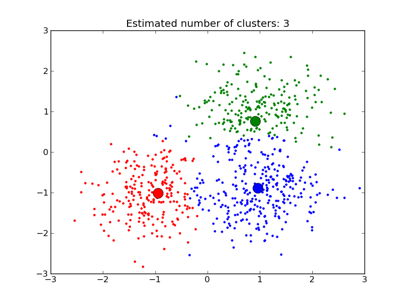
• Demo of affinity propagation clustering algorithm: Affinity Propagation on a synthetic 2D datasets with 3 classes.
• Finding structure in the stock market Affinity Propagation on Financial time series to find groups of companies

4.2.3. Mean Shift

MeanShift clusters data by estimating blobs in a smooth density of points matrix. This algorithm automatically sets its numbers of cluster. It will have difficulties scaling to thousands of samples.

Examples:

• A demo of the mean-shift clustering algorithm: Mean Shift clustering on a synthetic 2D datasets with 3 classes.

4.2.4. Spectral clustering

SpectralClustering does a low-dimension embedding of the affinity matrix between samples, followed by a KMeans in the low dimensional space. It is especially efficient if the affinity matrix is sparse and the pyamg module is installed. SpectralClustering requires the number of clusters to be specified. It works well for a small number of clusters but is not advised when using many clusters.

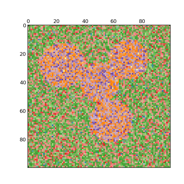
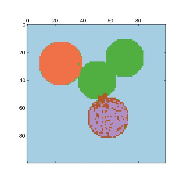
For two clusters, it solves a convex relaxation of the normalised cuts problem on the similarity graph: cutting the graph in two so that the weight of the edges cut is small compared to the weights in of edges inside each cluster. This criteria is especially interesting when working on images: graph vertices are pixels, and edges of the similarity graph are a function of the gradient of the image.

Examples:

• Spectral clustering for image segmentation: Segmenting objects from a noisy background using spectral clustering.
• Segmenting the picture of Lena in regions: Spectral clustering to split the image of lena in regions.

References:

• “A Tutorial on Spectral Clustering” Ulrike von Luxburg, 2007
• “Normalized cuts and image segmentation” Jianbo Shi, Jitendra Malik, 2000
• “A Random Walks View of Spectral Segmentation” Marina Meila, Jianbo Shi, 2001
• “On Spectral Clustering: Analysis and an algorithm” Andrew Y. Ng, Michael I. Jordan, Yair Weiss, 2001

4.2.5. Hierarchical clustering

Hierarchical clustering is a general family of clustering algorithms that build nested clusters by merging them successively. This hierarchy of clusters represented as a tree (or dendrogram). The root of the tree is the unique cluster that gathers all the samples, the leaves being the clusters with only one sample. See the Wikipedia page for more details.

The Ward object performs a hierarchical clustering based on the Ward algorithm, that is a variance-minimizing approach. At each step, it minimizes the sum of squared differences within all clusters (inertia criterion).

This algorithm can scale to large number of samples when it is used jointly with an connectivity matrix, but can be computationally expensive when no connectivity constraints are added between samples: it considers at each step all the possible merges.

4.2.5.1. Adding connectivity constraints

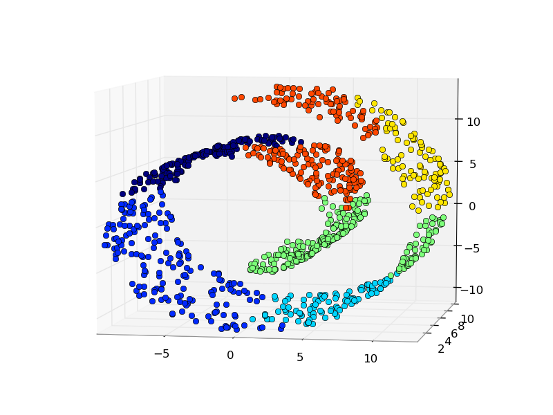
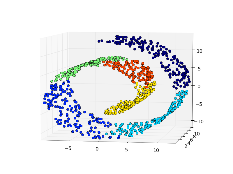
An interesting aspect of the Ward object is that connectivity constraints can be added to this algorithm (only adjacent clusters can be merged together), through an connectivity matrix that defines for each sample the neighboring samples following a given structure of the data. For instance, in the swiss-roll example below, the connectivity constraints forbid the merging of points that are not adjacent on the swiss roll, and thus avoid forming clusters that extend across overlapping folds of the roll.

The connectivity constraints are imposed via an connectivity matrix: a scipy sparse matrix that has elements only at the intersection of a row and a column with indices of the dataset that should be connected. This matrix can be constructed from apriori information, for instance if you whish to cluster web pages, but only merging pages with a link pointing from one to another. It can also be learned from the data, for instance using scikits.learn.neighbors.kneighbors_graph to restrict merging to nearest neighbors as in the swiss roll example, or using scikits.learn.feature_extraction.image.grid_to_graph to enable only merging of neighboring pixels on an image, as in the Lena example.

Examples:

• A demo of structured Ward hierarchical clustering on Lena image: Ward clustering to split the image of lena in regions.
• Hierarchical clustering: structured vs unstructured ward: Example of Ward algorithm on a swiss-roll, comparison of structured approaches versus unstructured approaches.
• Feature agglomeration vs. univariate selection: Example of dimensionality reduction with feature agglomeration based on Ward hierarchical clustering.