2.4.2. Machine Learning 101: General Concepts

Machine Learning is about building programs with tunable parameters (typically an array of floating point values) that are adjusted automatically so as to improve their behavior by adapting to previously seen data.

Machine Learning can be considered a subfield of Artificial Intelligence since those algorithms can be seen as building blocks to make computers learn to behave more intelligently by somehow generalizing rather that just storing and retrieving data items like a database system would do.

Decision boundary learned from two classes of data.

The following will introduce the main concepts used to qualify machine learning algorithms as implemented in scikit-learn:

• how to turn raw data info numerical arrays
• what is supervised learning
• what is unsupervised learning
• what is linearly separable data
• what is overfitting

2.4.2.1. Features and feature extraction

Most machine learning algorithms implemented in scikit-learn expect a numpy array as input X. The expected shape of X is (n_samples, n_features).

n_samples:The number of samples: each sample is an item to process (e.g. classify). A sample can be a document, a picture, a sound, a video, a row in database or CSV file, or whatever you can describe with a fixed set of quantitative traits. n_features:The number of features or distinct traits that can be used to describe each item in a quantitative manner.

The number of features must be fixed in advance. However it can be very high dimensional (e.g. millions of features) with most of them being zeros for a given sample. In this case we may use scipy.sparse matrices instead of numpy arrays so as to make the data fit in memory.

2.4.2.1.1. A simple example: the iris dataset

The machine learning community often uses a simple flowers database where each row in the database (or CSV file) is a set of measurements of an individual iris flower. Each sample in this dataset is described by 4 features and can belong to one of the target classes:

Features in the Iris dataset:  

0. sepal length in cm
1. sepal width in cm
2. petal length in cm
3. petal width in cm

Target classes to predict:  

0. Iris Setosa
1. Iris Versicolour
2. Iris Virginica

scikit-learn embeds a copy of the iris CSV file along with a helper function to load it into numpy arrays:

>>> from sklearn.datasets import load_iris
>>> iris = load_iris()

Note

To be able to copy and paste examples without taking care of the leading >>> and ... prompt signs, enable the ipython doctest mode with: %doctest_mode

The features of each sample flower are stored in the data attribute of the dataset:

>>> n_samples, n_features = iris.data.shape

>>> n_samples
150

>>> n_features
4

>>> iris.data[0]
array([ 5.1,  3.5,  1.4,  0.2])

The information about the class of each sample is stored in the target attribute of the dataset:

>>> len(iris.target) == n_samples
True

>>> iris.target
array([0, 0, 0, 0, 0, 0, 0, 0, 0, 0, 0, 0, 0, 0, 0, 0, 0, 0, 0, 0, 0, 0, 0,
       0, 0, 0, 0, 0, 0, 0, 0, 0, 0, 0, 0, 0, 0, 0, 0, 0, 0, 0, 0, 0, 0, 0,
       0, 0, 0, 0, 1, 1, 1, 1, 1, 1, 1, 1, 1, 1, 1, 1, 1, 1, 1, 1, 1, 1, 1,
       1, 1, 1, 1, 1, 1, 1, 1, 1, 1, 1, 1, 1, 1, 1, 1, 1, 1, 1, 1, 1, 1, 1,
       1, 1, 1, 1, 1, 1, 1, 1, 2, 2, 2, 2, 2, 2, 2, 2, 2, 2, 2, 2, 2, 2, 2,
       2, 2, 2, 2, 2, 2, 2, 2, 2, 2, 2, 2, 2, 2, 2, 2, 2, 2, 2, 2, 2, 2, 2,
       2, 2, 2, 2, 2, 2, 2, 2, 2, 2, 2, 2])

The names of the classes are stored in the last attribute, namely target_names:

>>> list(iris.target_names)
['setosa', 'versicolor', 'virginica']

2.4.2.1.2. Handling categorical features

Sometimes people describe samples with categorical descriptors that have no obvious numerical representation. For instance assume that each flower is further described by a color name among a fixed list of color names:

color in ['purple', 'blue', 'red']

The simple way to turn this categorical feature into numerical features suitable for machine learning is to create new features for each distinct color name that can be valued to 1.0 if the category is matching or 0.0 if not.

The enriched iris feature set would hence be in this case:

0. sepal length in cm
1. sepal width in cm
2. petal length in cm
3. petal width in cm
4. color#purple (1.0 or 0.0)
5. color#blue (1.0 or 0.0)
6. color#red (1.0 or 0.0)

2.4.2.1.3. Extracting features from unstructured data

The previous example deals with features that are readily available in a structured dataset with rows and columns of numerical or categorical values.

However, most of the produced data is not readily available in a structured representation such as SQL, CSV, XML, JSON or RDF.

Here is an overview of strategies to turn unstructed data items into arrays of numerical features.

Text documents:

Count the frequency of each word or pair of consecutive words in each document. This approach is called Bag of Words.

Note: we include other file formats such as HTML and PDF in this category: an ad-hoc preprocessing step is required to extract the plain text in UTF-8 encoding for instance.

Images:

• Rescale the picture to a fixed size and take all the raw pixels values (with or without luminosity normalization)

• Take some transformation of the signal (gradients in each pixel, wavelets transforms...)

• Compute the Euclidean, Manhattan or cosine similarities of the sample to a set reference prototype images aranged in a code book. The code book may have been previously extracted from the same dataset using an unsupervised learning algorithm on the raw pixel signal.

  Each feature value is the distance to one element of the code book.

• Perform local feature extraction: split the picture into small regions and perform feature extraction locally in each area.

  Then combine all the features of the individual areas into a single array.

Sounds:

Same strategy as for images within a 1D space instead of 2D

Practical implementations of such feature extraction strategies will be presented in the last sections of this tutorial.

2.4.2.2. Supervised Learning: model.fit(X, y)

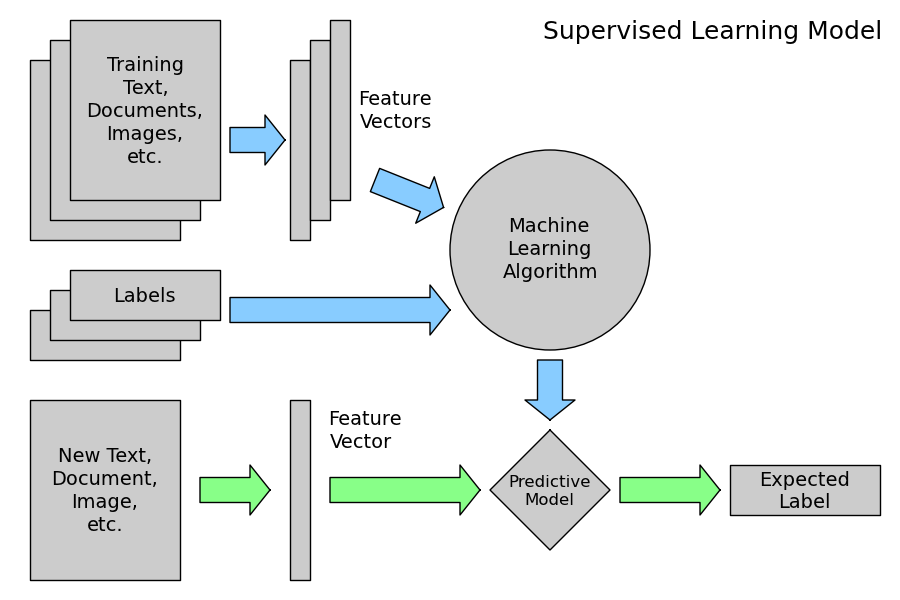
Supervised Learning overview

A supervised learning algorithm makes the distinction between the raw observed data X with shape (n_samples, n_features) and some label given to the model while training by some teacher. In scikit-learn this array is often noted y and has generally the shape (n_samples,).

After training, the fitted model does no longer expect the y as an input: it will try to predict the most likely labels y_new for new a set of samples X_new.

Depending on the nature of the target y, supervised learning can be given different names:

• If y has values in a fixed set of categorical outcomes (represented by integers) the task to predict y is called classification.
• If y has floating point values (e.g. to represent a price, a temperature, a size...), the task to predict y is called regression.

2.4.2.2.1. Classification

2.4.2.2.1.1. A first classifier example with scikit-learn

In the iris dataset example, suppose we are assigned the task to guess the class of an individual flower given the measurements of petals and sepals. This is a classification task, hence we have:

>>> X, y = iris.data, iris.target

Once the data has this format it is trivial to train a classifier, for instance a support vector machine with a linear kernel:

>>> from sklearn.svm import LinearSVC
>>> clf = LinearSVC(C=150)

Note

Whenever you import a scikit-learn class or function for the first time, you are advised to read the docstring by using the ? magic suffix of ipython, for instance type: LinearSVC?.

clf is a statistical model that has parameters that control the learning algorithm (those parameters are sometimes called the hyperparameters). Those hyperparameters can be supplied by the user in the constructor of the model. We will explain later how to choose a good combination using either simple empirical rules or data driven selection:

>>> clf
LinearSVC(C=150, class_weight=None, dual=True, fit_intercept=True,
     intercept_scaling=1, loss='l2', multi_class='ovr', penalty='l2',
     scale_C=True, tol=0.0001)

By default the real model parameters are not initialized. They will be tuned automatically from the data by calling the fit method:

>>> clf = clf.fit(X, y)

>>> clf.coef_                         
array([[ 0.18...,  0.45..., -0.80..., -0.45...],
       [ 0.05..., -0.89...,  0.40..., -0.93...],
       [-0.85..., -0.98...,  1.38...,  1.86...]])

>>> clf.intercept_                    
array([ 0.10...,  1.67..., -1.70...])

Once the model is trained, it can be used to predict the most likely outcome on unseen data. For instance let us define a list of simple sample that looks like the first sample of the iris dataset:

>>> X_new = [[ 5.0,  3.6,  1.3,  0.25]]

>>> clf.predict(X_new)
array([0], dtype=int32)

The outcome is 0 which is the id of the first iris class, namely ‘setosa’.

The following figure places the location of the fit and predict calls on the previous flow diagram. The vec object is a vectorizer used for feature extraction that is not used in the case of the iris data (it already comes as vectors of features):

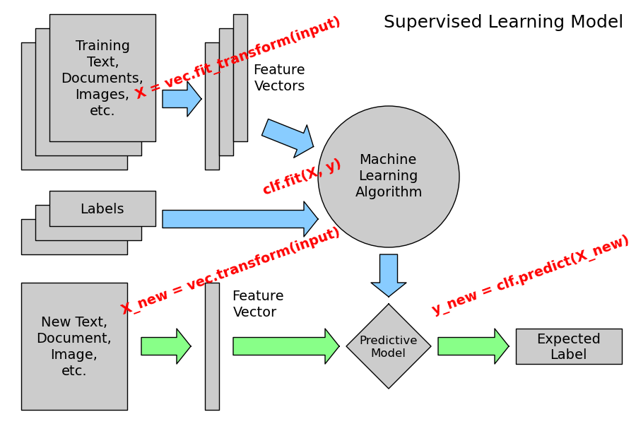
Supervised Learning with scikit-learn

Some scikit-learn classifiers can further predict probabilities of the outcome. This is the case of logistic regression models:

>>> from sklearn.linear_model import LogisticRegression
>>> clf2 = LogisticRegression(C=150).fit(X, y)
>>> clf2
LogisticRegression(C=150, class_weight=None, dual=False, fit_intercept=True,
          intercept_scaling=1, penalty='l2', scale_C=True, tol=0.0001)

>>> clf2.predict_proba(X_new)
array([[  9.07512928e-01,   9.24770379e-02,   1.00343962e-05]])

This means that the model estimates that the sample in X_new has:

• 91% likelyhood to belong to the ‘setosa’ class
• ~9% likelyhood to belong to the ‘versicolor’ class
• ~0% likelyhood to belong to the ‘virginica’ class

Of course, the predict method that outputs the label id of the most likely outcome is also available:

>>> clf2.predict(X_new)
array([0], dtype=int32)

2.4.2.2.1.2. Notable implementations of classifiers

sklearn.linear_model.LogisticRegression

Regularized Logistic Regression based on liblinear

sklearn.svm.LinearSVC

Support Vector Machines without kernels based on liblinear

sklearn.svm.SVC

Support Vector Machines with kernels based on libsvm

sklearn.linear_model.SGDClassifier

Regularized linear models (SVM or logistic regression) using a Stochastic Gradient Descent algorithm written in Cython

sklearn.neighbors.NeighborsClassifier

k-Nearest Neighbors classifier based on the ball tree datastructure for low dimensional data and brute force search for high dimensional data

sklearn.ensemble.ExtraTreesClassifier

A variant of Random Forests classifier: aggregation of many simple decision tree classifiers that each vote for the best class.

2.4.2.2.1.3. Sample application of classifiers

The following table gives examples of applications of classifiers for some common engineering tasks:

Task	Predicted outcomes
E-mail classification	Spam, normal, priority mail
Language identification in text documents	en, es, de, fr, ja, zh, ar, ru...
News articles categorization	Business, technology, sports...
Sentiment analysis in customer feedback	Negative, neutral, positive
Face verification in pictures	Same / different person
Speaker verification in voice recordings	Same / different person

2.4.2.2.2. Regression

Regression is the task of predicting the value of a continuously varying variable (e.g. a price, a temperature, a conversion rate...) given some input variables (a.k.a. the features, “predictors” or “regressors”). Some notable implementations of regression models in scikit-learn include:

sklearn.linear_model.Ridge

L2-regularized least squares linear model

sklearn.linear_model.ElasticNet

L1+L2-regularized least squares linear model trained using Coordinate Descent

sklearn.linear_model.LassoLARS

L1-regularized least squares linear model trained with Least Angle Regression

sklearn.linear_model.SGDRegressor

L1+L2-regularized least squares linear model trained using Stochastic Gradient Descent

sklearn.svm.SVR

Non-linear regression using Support Vector Machines (wrapper for libsvm)

sklearn.ensemble.ExtraTreesRegressor:

A variant of Random Forests applied to regression problems: aggregation of many simple decision tree trained for regression. The mean prediction of the trees is the prediction of the forest.

2.4.2.3. Unsupervised Learning: model.fit(X)

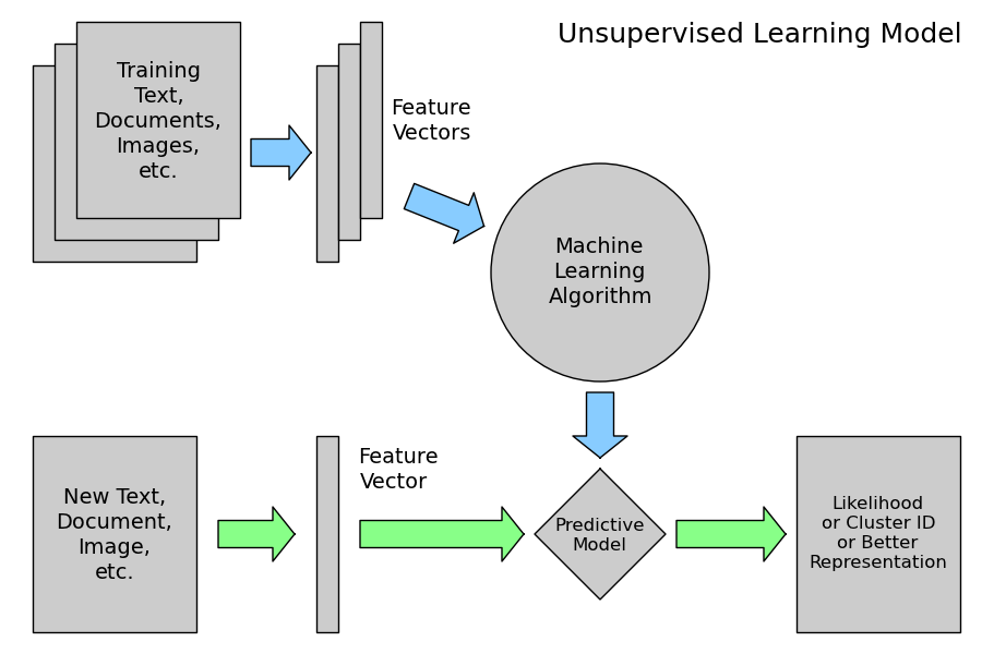
Unsupervised Learning overview

An unsupervised learning algorithm only uses a single set of observations X with shape (n_samples, n_features) and does not use any kind of labels.

An unsupervised learning model will try to fit its parameters so as to best summarize regularities found in the data.

The following introduces the main variants of unsupervised learning algorithms, namely dimensionality reduction and clustering.

2.4.2.3.1. Dimensionality Reduction and visualization

Dimensionality reduction is the task of deriving a set of new artificial features that is smaller than the original feature set while retaining most of the variance of the original data.

2.4.2.3.1.1. Normalization and visualization with PCA

The most common technique for dimensionality reduction is called Principal Component Analysis.

PCA can be done using linear combinations of the original features using a truncated Singular Value Decomposition of the matrix X so as to project the data onto a base of the top singular vectors.

If the number of retained components is 2 or 3, PCA can be used to visualize the dataset:

>>> from sklearn.decomposition import PCA
>>> pca = PCA(n_components=2, whiten=True).fit(X)

Once fitted, the pca model exposes the singular vectors in the components_ attribute:

>>> pca.components_                                      
array([[ 0.17..., -0.04...,  0.41...,  0.17...],
       [-1.33..., -1.48...,  0.35...,  0.15...]])

>>> pca.explained_variance_ratio_                        
array([ 0.92...,  0.05...])

>>> pca.explained_variance_ratio_.sum()                  
0.97...

Let us project the iris dataset along those first 3 dimensions:

>>> X_pca = pca.transform(X)

The dataset has been “normalized”, which means that the data is now centered on both components with unit variance:

>>> import numpy as np
>>> np.round(X_pca.mean(axis=0), decimals=5)
array([-0.,  0.])

>>> np.round(X_pca.std(axis=0), decimals=5)
array([ 1.,  1.])

Furthermore the samples components do no longer carry any linear correlation:

>>> import numpy as np
>>> np.round(np.corrcoef(X_pca.T), decimals=5)
array([[ 1., -0.],
       [-0.,  1.]])

And visualize the dataset using pylab, for instance by defining the following utility function:

>>> import pylab as pl
>>> from itertools import cycle
>>> def plot_2D(data, target, target_names):
...     colors = cycle('rgbcmykw')
...     target_ids = range(len(target_names))
...     pl.figure()
...     for i, c, label in zip(target_ids, colors, target_names):
...         pl.scatter(data[target == i, 0], data[target == i, 1],
...                    c=c, label=label)
...     pl.legend()
...     pl.show()
...

Calling plot_2D(X_pca, iris.target, iris.target_names) will display the following:

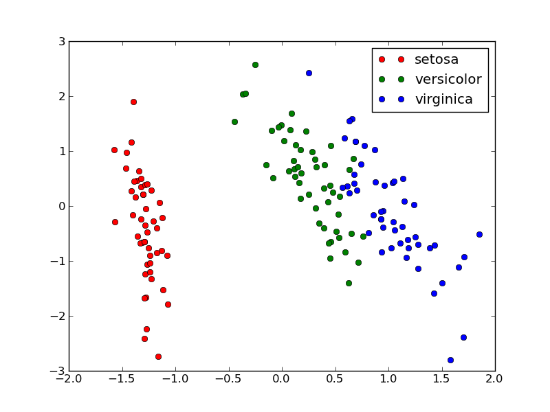
2D PCA projection of the iris dataset

Note

scikit-learn also provides implementation for various manifold_learning algorithm that might render more interesting visualization than PCA on complex data.

2.4.2.3.1.2. Other applications of dimensionality reduction

Dimensionality Reduction is not just useful for visualization of high dimensional datasets. It can also be used as a preprocessing step (often called data normalization) to help speed up supervised machine learning methods that are not computationally efficient with high n_features such as SVM classifiers with gaussian kernels for instance or that do not work well with linearly correlated features.

Note

The default implementation of PCA computes the SVD of the full data matrix, which is not scalable when both n_samples and n_features are big (more that a few thousands).

If you are interested in a number of components that is much smaller than both n_samples and n_features, consider using sklearn.decomposition.RandomizedPCA instead.

2.4.2.3.2. Clustering

Clustering is the task of gathering samples into groups of similar samples according to some predefined similarity or dissimilarity measure (such as the Euclidean distance).

For instance let us reuse the output of the 2D PCA of the iris dataset and try to find 3 groups of samples using the simplest clustering algorithm (KMeans):

>>> from sklearn.cluster import KMeans
>>> from numpy.random import RandomState
>>> rng = RandomState(42)

>>> kmeans = KMeans(3, random_state=rng).fit(X_pca)

>>> np.round(kmeans.cluster_centers_, decimals=2)
array([[ 1.02, -0.71],
       [ 0.33,  0.89],
       [-1.29, -0.44]])

>>> kmeans.labels_[:10]
array([2, 2, 2, 2, 2, 2, 2, 2, 2, 2])

>>> kmeans.labels_[-10:]
array([0, 0, 1, 0, 0, 0, 1, 0, 0, 1])

We can plot the assigned cluster labels instead of the target names with:

plot_2D(X_pca, kmeans.labels_, ["c0", "c1", "c2"])

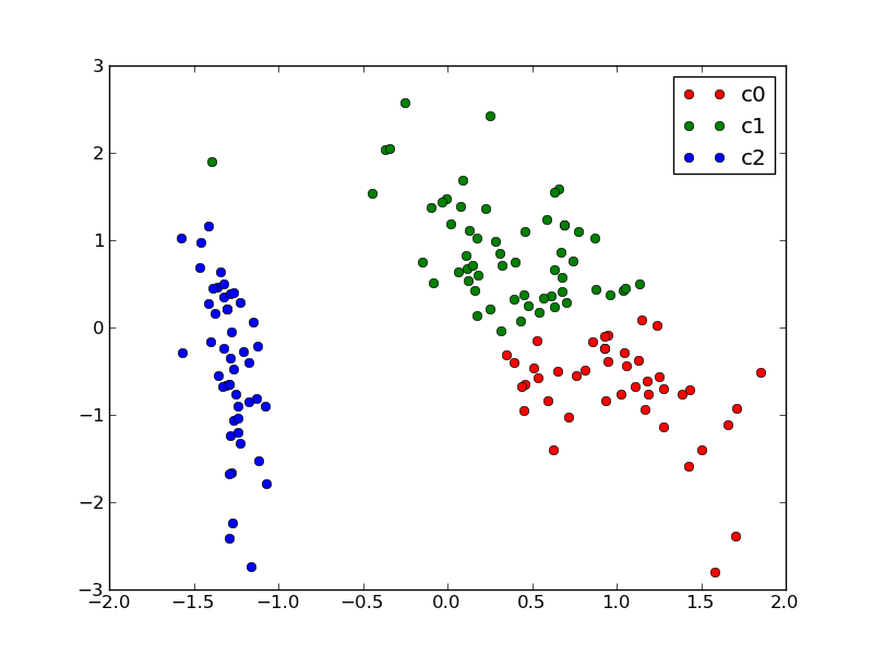
KMeans cluster assignements on 2D PCA iris data

2.4.2.3.2.1. Notable implementations of clustering models

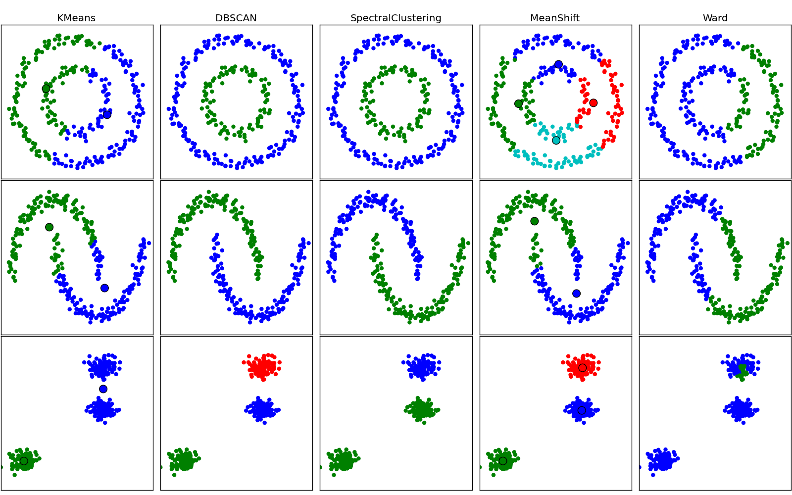
The following are two well-known clustering algorithms. Like most unsupervised learning models in the scikit, they expect the data to be clustered to have the shape (n_samples, n_features):

sklearn.cluster.KMeans and sklearn.cluster.MiniBatchKMeans

The simplest, yet effective clustering algorithm. Needs to be provided with the number of clusters in advance, and assumes that the data is normalized as input (for instance using sklearn.preprocessing.Scaler or sklearn.decomposition.PCA as preprocessor).

sklearn.cluster.MeanShift

Can find better looking clusters than KMeans but is not scalable to a high number of samples.

sklearn.cluster.DBSCAN

Can detect irregularly shaped clusters based on density, i.e. sparse regions in the input space are likely to become inter-cluster boundaries. Can also detect outliers (samples that are not part of a cluster).

sklearn.cluster.Ward

Hierarchical clustering computes a minim spanning tree between samples and cut it to find the required number of cluster. This can give good results on small to medium dataset. It further give the ability to give connectivity constraints between the samples.

Other clustering algorithms do not work with a data array of shape (n_samples, n_features) but directly with a precomputed affinity matrix of shape (n_samples, n_samples):

sklearn.cluster.AffinityPropagation

Clustering algorithm based on message passing between data points.

sklearn.cluster.SpectralClustering

KMeans applied to a projection of the normalized graph Laplacian: finds normalized graph cuts if the affinity matrix is interpreted as an adjacency matrix of a graph.

DBSCAN can work with either an array of samples or an affinity matrix.

2.4.2.3.2.2. Applications of clustering

Here are some common applications of clustering algorithms:

• Building customer profiles for market analysis
• Grouping related web news (e.g. Google News) and websearch results
• Grouping related stock quotes for investment portfolio management
• Can be used as a preprocessing step for recommender systems
• Can be used to build a code book of prototype samples for unsupervised feature extraction for supervised learning algorithms

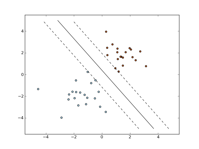
2.4.2.4. Linearly separable data

Some supervised learning problems can be solved by very simple models (called generalized linear models) depending on the data. Others simply don’t.

To grasp the difference between the two cases, run the interactive example from the examples folder of the scikit-learn source distribution:

% python $SKL_HOME/examples/applications/svm_gui.py

1. Put some data points belonging to one of the two target classes (‘white’ or ‘black’) using left click and right click.
2. Choose some parameters of a Support Vector Machine to be trained on this toy dataset (n_samples is the number of clicks, n_features is 2).
3. Click the Fit but to train the model and see the decision boundary. The accurracy of the model is displayed on stdout.

The following figures demonstrate one case where a linear model can perfectly separate the two classes while the other is not linearly separable (a model with a gaussian kernel is required in that case).

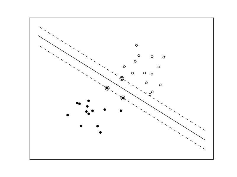
Linear Support Vector Machine trained to perfectly separate 2 sets of data points labeled as white and black in a 2D space.

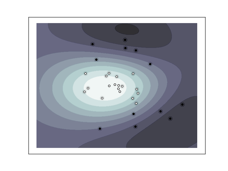
Support Vector Machine with gaussian kernel trained to separate 2 sets of data points labeled as white and black in a 2D space. This dataset would not have been seperated by a simple linear model.

Exercise:

Fit a model that is able to solve the XOR problem using the GUI: the XOR problem is composed of 4 samples:

• 2 white samples in the top-left and bottom-right corners
• 2 black samples in the bottom-left and top-right corners

Question: is the XOR problem linearly separable?

Exercise:

Construct a problem with less than 10 points where the predictive accuracy of the best linear model is 50%.

2.4.2.5. Training set, test set and overfitting

The most common mistake beginners do when training statistical models is too overestimate the predictive performance of their model by computing the accurracy on the dataset used to train the model.

Never measure the quality of the model on the training dataset!

2.4.2.5.1. The overfitting issue

The problem lies in the fact that some models can be subject to the overfitting issue: they can learn the training data by heart without generalizing. The symptoms are:

• the predictive accurracy on the data used for training can be excellent (sometimes 100%)
• however, the models do little better than random prediction when facing new data that was not part of the training set

If you evaluate your model on your training data you won’t be able to tell whether your model is overfitting or not.

2.4.2.5.2. Solutions to overfitting

The solution to this issue is twofold:

1. Split your data into two sets to detect overfitting situations:

• one for training and model selection: the training set
• one for evaluation: the test set

2. Avoid overfitting by using simpler models (e.g. linear classifiers instead of gaussian kernel SVM) or by increasing the regularization parameter of the model if available (see the docstring of the model for details)

When the amount of labeled data available is small, it may not be feasible to construct training and test sets. In that case, use cross validation: divide the dataset into ten parts of (roughly) equal size, then for each of these ten parts, train the classifier on the other nine and test on the held-out part.

2.4.2.5.3. Measuring classification performance on a test set

Here is an example on you to split the data on the iris dataset using the sklearn.cross_validation.train_test_split helper function:

>>> from sklearn.cross_validation import train_test_split

This function will split any dataset by applying random shuffling and selecting a fraction of the sample as held out test set:

>>> X_train, X_test, y_train, y_test = train_test_split(
...    iris.data, iris.target, test_fraction=0.333, random_state=42)

>>> X_train.shape
(100, 4)

>>> X_test.shape
(50, 4)

>>> y_train.shape
(100,)

>>> y_test.shape
(50,)

We can now re-train a new linear classifier on the training set only:

>>> clf = LinearSVC(C=150).fit(X_train, y_train)

To evaluate its quality we can compute the average number of correct classifications on the test set:

>>> np.mean(clf.predict(X_test) == y_test)              
0.979...

This shows that the model has a predictive accurracy very close to 100% which means that the classification model was capable of generalizing what was learned from the training set to the test set: this is rarely so easy on real life datasets as we will see in the following chapter.

2.4.2.5.4. Measuring performance using cross-validation

The simple train / test split gives one value the impact of the random shuffling and split is unknown. To get a better idea of the variance of the generalization score one can repeat the process several times using cross-validation.

Let’s build a new, untrained classifier:

>>> clf = LinearSVC(C=150)

We can use the sklearn.cross_validation.cross_val_score utility to perform Cross-Validation in a single call:

>>> from sklearn.cross_validation import cross_val_score
>>> scores = cross_val_score(clf, X, y, cv=10)
>>> scores
array([ 1.        ,  0.86666667,  0.93333333,  1.        ,  1.        ,
        0.86666667,  0.93333333,  1.        ,  1.        ,  1.        ])

This generalization performance can be summarized by the mean and standard deviation:

>>> scores.mean(), scores.std()                         
(0.959..., 0.053...)

There are many ways to do cross-validation, more details available in the Cross-Validation section of the documentation.

2.4.2.6. Key takeaway points

• Build X (features vectors) with shape (n_samples, n_features)
• Supervised learning: clf.fit(X, y) and then clf.predict(X_new)
  • Classification: y is an array of integers
  • Regression: y is an array of floats
• Unsupervised learning: clf.fit(X)
  • Dimensionality Reduction with clf.transform(X_new)
    • for visualization
    • for scalability
  • Clustering finds group id for each sample
• Some models work much better with data normalized with PCA but also simpler Preprocessing data schemes such as centering and variance scaling.
• Simple linear models can fail completely (non linearly separable data)
• Simple linear models often very useful in practice (esp. with large n_features)
• Before starting to train a model: split train / test data:
  • Use training set for model selection and fitting.
  • Use test set for model evaluation.
  • Use cross-validation when your dataset is small.
• Complex models can overfit (learn by heart) the training data and fail to generalize correctly on test data:
  • Try simpler models first.
  • Tune the regularization parameter on a development set.